Time Series Scalar Data
Time-series data files for sensors collecting one-dimensional data are described here (i.e., every time-stamped data record refers to a value at a single point in space). This definition may include instruments on mobile platforms such as Wally (a crawler in Barkley Canyon) or the Vertical Profiling System (VPS), for more information see the mobile device page. However, gridded data from instruments like multibeam sonar and echosounders are excluded. For data searches defined by location and data source, (e.g. CTD at Folger Deep), new files will not be made if the device contributing the data is modified, (i.e. if the CTD is swapped for another). For data searches defined by instrument type, (e.g. CTD 10600), if the device is moved (e.g. from MTC to Folger Deep), new files will be made.
Four formats of Time Series Scalar Data are currently offered: CSV (comma-separated variables), JSON (javascript object notation), ODV (Ocean Data View) and MAT (matlab). CSV, JSON and ODV are text format files readable by any text editor or text-reading capable software. MAT format files are readable by Mathworks Matlab. A prototype NetCDF format exists but is not yet offered to all users. NetCDF is also available from our ERDDAP server. User requests for additional formats will be seriously considered (we're always happy to help), please contact us.
Oceans 3.0 API filter: dataProductCode=TSSD
Revision History
- 20221125: Min/max and min/max+avg added to resampling options
- 20220301: sensor-level data ratings added
- 20170401: JSON format files added
- 20131003: Ocean Data View Spreadsheet TXT files added
- 20130725: Data product options implemented, merged in CSV-NaN data product
- 20130320: Improved support of varying sample periods, integration of QAQC flags
- 20120626: Station search fully supported, so that file breaks are not made when the devices change
- 20110912: Subsampled data products modified to extend query time range such that it has exact subsample period endpoints
- 20110823: CSVs modified to contain up to 1 million records per file, header slightly modified
- 20101130: 1 minute interval added to subsampling options
- 20100513: Subsampling option introduced
- 20091208: Data product initially released
See New Features Release Notes for more updates
Data Product Options
Quality Control
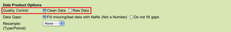
Raw Data
When this option is selected, raw data will be supplied in the data products: no action is taken to modify the data. In general, all scalar data is associated with a quality control flag. These flags are stored adjacent to the data values.
Oceans 3.0 API filter: dpo_qualityControl=0
Clean Data
Selecting this option will cause any data values with quality control failures (QAQC flags 3, 4 and 6) to be replaced with NaNs. If the do not fill data gaps option is selected, data values with quality control failures will be removed. For all data products, when resampling with the clean option, any data with quality control failures are removed prior to the resampling (this rule applies to all resampling types: average, min/max, etc).
This is the default option for all data products.
Oceans 3.0 API filter: dpo_qualityControl=1
File-name mode field
'clean' is added to the file-name when the quality option is set to clean data.
Data Gaps
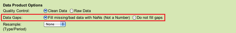
Fill missing/bad data with NaNs (Not Number)
This option will, as it says, fill in data gaps with 'NaN' values in the data products. For CSV files, the text 'NaN' is inserted, while MAT files have a built-in type of the same name. Data gaps occur when the time difference between subsequent readings is greater than 1.9 times the sample period (otherwise known as the data rating). The NaNs are placed one sample period after the last reading before the data gaps. Gaps are only filled between readings.
This option will also keep any existing NaNs in the data. These are most often caused by the clean data option being selected, or by real NaNs being report, or when a sensor in a multi-sensor data product has no data. Available metadata can elaborate on the QAQC test that was applied (this information is available via Oceans 3.0 and in MAT files).
This is the default option.
Oceans 3.0 API filter: dpo_dataGaps=1
Do not fill gaps
This option will not take action to fill in data gaps.
This option will cause action to be taken to remove all NaNs in the data. The main implication of this is if the clean option had been selected, data that failed quality control tests will be removed entirely. However, there is an exception to this: for multi-sensor time series scalar data, if one sensor at a given time stamp has valid data, the entire row/time stamp cannot be removed, so the remaining sensors will be left as NaNs. For clarification, see the following example, note that QAQC flags of 1s are good data, 4s are failures and 9s are missing data:
sample time | sensor 1 | sensor 1 flag | sensor 2 | sensor 2 flag | Comment |
|---|---|---|---|---|---|
12:00:00 | 42 | 1 | 42 | 1 | Good row. |
12:00:01 | NaN | 4 | NaN | 9 | Two bad values; one QAQC failure, one data gap. If the do not fill gaps is selected, this entire row will be removed. |
12:00:02 | NaN | 4 | 44 | 1 | One good value, can't remove row. |
File-name mode field
'NaN' is added to the file name when the data gaps are filled with NaNs.
Oceans 3.0 API filter: dpo_dataGaps=0
Resampling
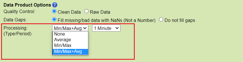
Resample Type:
None - no resampling. This is the default option for time series scalar data.
Oceans 3.0 API filter:
dpo_resample=none
Average - the mean value within resample period (fixed-window averaging without overlap). This is also known as a 'box-car' or ensemble average. It is subject to the 70% data completeness QAQC check (see below) with the exception of engineering data or data from irregular or scheduled sampling. Only available with the clean data product option.
Oceans 3.0 API filter:
dpo_resample=averageMin/Max - the most extreme minimum and maximum values within resample period. It is subject to the 70% data completeness QAQC check (except for engineering data or data from irregular or scheduled sampling); QAQC flags are taken from the extreme data points.
Oceans 3.0 API filter:
dpo_resample=minMaxanddpo_minMax={0, 60, 600, 900, 3600, 86400}Min/Max+Avg - the combination of the min/max and average as described above. The average is always calculated from clean data and will be NaN if there is less than 70% data available after cleaning. QAQC flags for min/max+avg with automatic resampling are the worst flag in the resample period, which includes the 70% check on data completeness (except for engineering data or data from irregular or scheduled sampling). This is the default option for time series scalar plots - other plots, such as the BHT, AGO, profile or staircase plots will have different options and defaults.
Oceans 3.0 API filter:
dpo_resample=minMaxAvganddpo_minMaxAvg={0, 60, 600, 900, 3600, 86400}
Resample Period:
Visible when an actionable resample type is selected, immediately to the right of the resample type. Current periods offered:
1 Minute:
Oceans 3.0 API filter:
dpo_average=6010 Minute:
Oceans 3.0 API filter:
dpo_average=60015 Minute:
Oceans 3.0 API filter:
dpo_average=9001 Hour:
Oceans 3.0 API filter:
dpo_average=36001 Day:
Oceans 3.0 API filter:
dpo_average=86400
When resampling is selected:
- The timestamps in the data series correspond to the centre of each resampling interval. (Data downloaded prior to 13 Feb 2013: timestamps were at beginning of interval). The resample interval always begins and ends at an integer multiple of the resample period, so minutes on the minute, hours on the hour, days on the day, etc.
- If the date/time range on the search has limits that are within a resampling interval, the date/time endpoints are extended to include the entire resampling interval. For example, when daily resampling is selected from 03:00:00.000 on Monday to 20:00:00.000 on Thursday, the date range is extended to 00:00:00.000 on Monday to 23:59.59.999 on Thursday.
- Note that tides are not filtered out in resampled products.
- No anti-alias filtering is done. This is why only averaging and min/max are offered at this time. Box-car / ensemble averaging is an easily understood and ubiquitous process that is an effective low-pass anti-alias filter. For more information, see this page on data reduction and time-averaging.
- Spatial / mobile data may be resampled, but users are warned against this procedure, as it may be inappropriate to do so. Spatial averages or a geospatial display of the non-resampled data may be a better approach.
- All resampled data products are subject to an additional QAQC check on data completeness (except engineering data or data from irregular or scheduled sampling). If any resample period does not contain at least 70% of the expected data, the QAQC flag for this period will be a failure (6), unless overridden by a manual QAQC flag, see the QAQC page. For live data, it is quite likely that the last resample period will not be complete and will be flagged; this is especially obvious for plots. Future improvements will allow users to modify the data completeness threshold.
More options will be available in the future as we work to improve the data products. Feedback is welcomed and encouraged. For custom resampling, users can develop their own matlab code in the Oceans 3.0 Sandbox and run it in the ONC computing environment.
File-name mode field
The resample type and period are added to the file-name when resampling is selected. Example: 'avg1hour', 'MinMax10minute'.
JSON Output Encoding
Applies to JSON format files only.
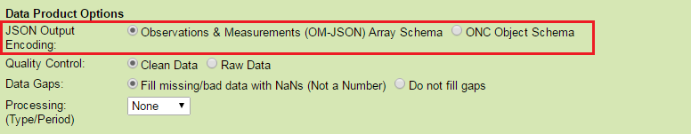
Observations & Measurements (OM – JSON) Array Schema
Data will be output as three arrays for each sensor: sampleTime, values, qaqcFlags.
Oceans 3.0 API filter: dpo_jsonOutputEncoding=OM
ONC Object Schema
Data will be output as a list of objects for each sensor. Inside each data object, there are single values of sampleTime, value, and qaqcFlag.
Oceans 3.0 API filter: dpo_jsonOutputEncoding=ONC
File-name mode field
"OM" or "ONC" will appear last in the file-name mode, immediately prior to the ".json" file extension.
Formats
This data is available in CSV, JSON, ODV and MAT formats, plus a prototype netCDF format that is only accessible for internal users. Content descriptions and example files are provided below. A new file is started whenever an instrument has new coordinates (lat, lon, depth). See the mobile device page to see how these data products handle data from mobile devices.
CSV (Comma Separated Variables)
CSV-formatted data files can be opened with Microsoft Excel, Ocean Data View, R, SPSS, Minitab, Matlab, text editors or any other software capable of reading delimited text files. Each file is limited to a maximum of 1 million records.
Files are divided into sections for metadata and data. All non-data entries are preceded by the pound sign (#). Sub-sections are delimited by dashed-lines. Each section and its contents are described here, and a sample can be found below.
- Creation Date: Date and time (using ISO8601 format) that the data product was produced. This is a valuable indicator for comparing to other revisions of the same data product.
Origin Section
- SOURCE: Citation author.
- HTTP: Citation publication site.
- HOME: Citation publication location.
- FLDATE: Creation date of the file.
- CITATION1: the DOI citation text as it appears on the Dataset Landing Page. If the file contains data from multiple datasets, additional lines of CITATION will follow (CITATION2, CITATION3, etc.)
- METADATF: Metadata file name.
- SEARCHID: DMAS search ID from Oceans2.0.
Location Section
- STNNAME: Station name.
- STNCODE: Station code.
- LATITUDE: Latitude north.
- LONGITUDE: Longitude east.
- DEPTH: Obtained at time of deployment (m).
Device Section
- DEVCAT: Device category.
- DEVTOT: Total number of device deployments contributing to data.
- DEPLDATE: Device deployment date.
- DEVNAME: Full device name.
- DEVCODE: Device code.
- DEVID: Device ID.
Data Section
- DATEFROM: First timestamp (using ISO8601 format) contained within the time series.
- DATETO: Last timestamp (using ISO8601 format) contained within the time series.
- PERIODTOT: Total number of sample periods for the device-level sample period(s).
- PERIODST1: Device-level sample period start time. This row and PERIOD# row is repeated for additional device-level sample periods.
- PERIOD1: Device-level sensor sample period (s).
- SENSOR1NAME: Name of sensor for the following sensor-level sample periods (if any). This row and SENSOR#PERIODTOT is repeated for each sensor that has a sensor-level data rating / sample period.
- SENSOR1PERIODTOT: Number of sample period / start time pairs that appear below for the sensor named above.
- SENSOR1PERIODST1: Sensor-level sample period start time for this sensor and start time. This row and SENSOR#PERIOD# is repeated for each sample period for this sensor.
- SENSOR1PERIOD1: Sensor-level sample period for this sensor and start time.
- RESAMPPRD: Re/subsample time in seconds.
- RESAMPTYP: As selected via the data search.
- RESAMPMIN: Minimum percent valid data per resample.
- RESAMPDCR: Description of subsample type.
- TOTSAMPLE: Total number of data samples in the file.
- TOTSMPEXP: Total number of expected samples for the date range.
- DPOPTGAPS: Data product option selected for data gaps: fill or remove missing data.
- DPOPTQC: Data product option to select clean or raw data.
- QAREMARK: Quality assurance remarks.
EXAMPLE FILE: CambridgeBay_UnderwaterNetwork_ConductivityTemperatureDepth_20180701T000000Z_20180701T005958Z-NaN_clean.csv
Oceans 3.0 API filter: extension=csv
CSV with NaNs
When the 'Fill data gaps with NaNs (Not A Number)' is selected, the time series scalar data products add lines of NaNs for missing samples or empty resample periods to fill the gap in the data, as described in the data gaps section.
For example, a regular Time Series Scalar CSV file for an instrument with 4 sensors might contain the following for an instrument with a one second sampling period: (QAQC flags are excluded for this example)
20120206T000000.000Z,45.34,0.01,NaN,2543
20120206T000001.001Z,45.53,0.01,NaN,2542
20120206T000006.045Z,46.01,0.01,NaN,2541
while the same data for a CSV with NaNs would contain the following
20120206T000000.000Z,45.34,0.01,NaN,2543
20120206T000001.001Z,45.53,0.01,NaN,2542
20120206T000002.001Z,NaN,NaN,NaN,NaN
20120206T000003.001Z,NaN,NaN,NaN,NaN
20120206T000004.001Z,NaN,NaN,NaN,NaN
20120206T000005.001Z,NaN,NaN,NaN,NaN
20120206T000006.045Z,46.01,0.01,NaN,2541
In the first example, there was a data gap of four sample periods between the second and third lines. This shows up in the CSV with NaNs as four lines of NaNs. In both cases, NaNs was written into the fourth column. This is because no data was found for that sensor for any of the timestamps.
This data product was created for users that are opening their CSV data within an application that requires the NaN-valued time stamps in order to graph the data properly.
The timestamps for the rows of NaN-values are calculated programmatically as follows:
- Determine the gap size in milliseconds.
- Determine the number of missing time stamps in that gap.
- For each missing timestamp, increment by one sample period. In the example above, the timestamps were incremented by one second.
If there is any clock drift on the instrument, there may be a noticeable jump between the last timestamp in the data-gap and the one immediately following, but it should never be more or less than two sample periods.
JSON
JSON-formatted data files can be opened with many text editors or any other software capable of parsing JSON format. Each file is limited to a maximum of one hundred thousand records.
Files contain two main objects: metadata and sensorData (one object per sensor). metadata contains the same metadata as the CSV file header, whereas sensorData differs from the CSV data section by having additional fields such as sensorName, unitofMeasure and actualSamples. See the CSV documentation above for more information on each field - the same definitions and java-code engine are used to generate both CSV and JSON. JSON files can be downloaded in two different formats as noted in the Data Product Options. The only difference between these two formats is the output of data field in sensorData.
Here is the generalized JSON structure for both OM and ONC format JSON:
"metadata": {
      "dataSection": {
         "dataProductOptionGap": string,
         "dataProductOptionQualityControl": string,
         "dataQualityAssuranceRemark": string,
         "dateFrom": string,
         "dateTo": "string,
         "minPercentValidData": string,
         "resampleDescription": string,
         "resamplePeriod": string,
         "resampleType": string,
         "samplePeriodTotal": integer,
         "samplePeriods": [
            {
               "samplePeriod": integer,
               "samplePeriodStartTime": string
            }
         ],
         "totalSample": integer,
         "totalSampleExpected": integer
      },
      "deviceSection": {
         "deploymentTotal": integer,
         "deviceCategory":  string,
         "deviceDeployments": [
            {
               "deploymentDate": string,
               "deviceCode": string,
               "deviceId": integer,
               "deviceName": string
            }
         ]
      },
      "locationSection": {
         "depth": double,
         "latitude": double,
         "longitude": double,
         "stationCode": string,
         "stationName": string
      },
      "originSection": {
         "citations": string,
         "creationDate": string,
         "http": string,
         "metadataFileName": string
         "searchId": integer,
         "source": string
      }
   }
sensorData": [
      {
         "actualSamples": integer,
         "sensor": string,
         "sensorName": string,
         "unitOfMeasure": string,

         "data": [// for ONC-JSON (standard object-based)
            {
            "sampleTime": string,
            "value": double,
            "qaqcFlag": integer
            },
         ...
         "data": [ // for OM-JSON (Observations & Measurements)
            {
            "sampleTime": [array of strings],
            "value": [array of doubles],
            "qaqcFlag": [array of integers]
            },
          ]
      },
   ]
}
When resampling is selected, additional fields are added, such as 'counts' for the number of samples in the resample (average, min/max) period as well as fields for the min and max values, times at min/max, flags at min/max.
Oceans 3.0 API filter: extension=json
TXT (Ocean Data View Spreadsheet File)
Ocean Data View (ODV) spreadsheet files are plain text (ASCII) semi-colon delimited files similar to CSV files described above. They can be opened by Ocean Data View, R, SPSS, Minitab, Matlab, Microsoft Excel, text editors or any other software capable of reading delimited text files. Ocean data view can open/import this format without any additional user input and the data is instantly available for visualization. MS Excel users can view the file easily by importing with the delimiter set to a semi-colon. Each file is limited to a maximum of 1 million records (for compatibility with MS Excel).
ODV text files have three main parts: the file header, containing metadata, the data header and the data body. The data body contains the same data as a CSV file with additional metadata columns that Ocean Data Views uses to break up multiple deployments (for instance if instruments are swapped out, Ocean Data View will show this as separate stations). The file header has a fixed number of rows (it will grow horizontally with additional data), making it easy to handle in statistical packages like R. The field definitions provided below are the same as the MAT format data product (below) as both are generated by the matlab scalar data engine.
File Header
The file header contains the same information as the CSV header, with additional fields. All time data listed is in ISO 8601 format with dashes and colons; the time base is UTC or 'zulu' time, which is what the 'Z' following all the time stamps indicates. The header is structured with a comment marker '//' preceding every row, with data contained within XML-like tags that describe the data. For example, the first line of the header will normally be this:
//<Creator>Ocean Networks Canada - University of Victoria</Creator>
Additional important fields include:
- CreateTime - the time that the file was created.
- Citation - a single line with a citation for each dataset / deployment, ordered by date, separated by comma. Each citation consists of the DOI citation text as it appears on the Dataset Landing Page. The citation text is formatted as follows: <Author(s) in alphabetical order>. <Publication Year>. <Title, consisting of Location Name (from searchTreeNodeName or siteName in ONC database) Deployed <Deployment Date (sitedevicedatefrom in ONC database)>. <Repository>. <Persistent Identifier, which is either a DOI URL or the queryPID (search_dtlid in ONC database)>. Accessed Date <query creation date (search.datecreated in ONC database)>
- DeviceDeployment - this is the time range of each deployment in a comma separated list. Each deployment is defined in the following fields: Location, SiteName, DeviceName, DeviceCode, Latitude, Longitude, Depth. In most cases, there will be only one device deployment listed. However, the likelihood of multiple deployments increases if the location search time range spans our maintenance season (June-September) when devices are swapped or redeployed.
- SamplePeriod, SampleSize, SamplePeriodDateFrom, SamplePeriodDateTo, SamplePeriodSensorName - these fields contain all of the sample period information that is applicable to the data found. (This is a different format than the presentation in the CSV file). Each field has the same length with each value corresponding by index to the other fields's values. Sample periods are grouped by sensor name, indicated by a comma, so that every sensor in the file has a complete record of it's sample period.
- SamplesReceived, SamplesExpected - this is a summary of the number data samples in the file and number expected, after resampling/cleaning. Filled values don't count.
- DataProductOptions - summarizes the options choosen for the data product, including quality control filtering, data gaps and resampling.
- QC - this field describes the QAQC flags used. For ODV spreadsheet files only, the flag scheme is the ARGO standard adapted by ODV. ONC and ARGO flags are essentially identical with the exception that ONC uses flag 7 to represent averaged data. To conform to the ARGO scheme, any flags with a value of 7 are replaced with 1, where flag 1 is 'good data' and flag 7 is 'good averaged data'. The transformation from our flag scheme to ARGO and ODV flags can be found at the top of the QAQC page. Here is ODV's description of the available flag schemas: ODV4_QualityFlagSets.pdf. Note that ARGO flags are only supported in ODV version 4 and above.
- DataQualityComment: In some cases, there are particular quality-related issues that are mentioned here. This is distinct from QAQC information mentioned above.
Data Header
The data header is the column headings for the data body. It contains headings like the following example. The top row is the column headings stripped of data format tags, the second row is a description of the headings, the third row is an example row of data.
Type | Cruise | Station | yyyy-mm-ddThh:mm:ss.sss | Latitude [degrees_north] | Longitude [degrees_east] | time_ISO8601 | Seafloor Pressure [decibar] | QV:ARGO:Seafloor Pressure [decibar] |
|---|---|---|---|---|---|---|---|---|
Blank | Device Name (ID number) | Site-Device Name (ID number) | Site-Device start time | (for the Site-Device) | (for the Site-Device) | time of data reading - primary variable | data value - dependent variable | ARGO QAQC Flag |
* | NRCan Bottom Pressure Recorder 5 (22790) | Deep_BPR_2011-07 (100150) | 2013-09-09T23:10:08.222 | 48.814 | -125.281 | 2013-09-09T23:10:08.222 | 107.237646131 | 1 |
Here is an example file for one hour of data: CambridgeBay_UnderwaterNetwork_ConductivityTemperatureDepth_20180701T000000Z_20180701T005958Z-NaN_clean_ODV.txt
Resampled ODV txt files will also contain a variable containing the count of the data points that contributed to the resampled value (average and/or min/max). When averaging, the standard deviation is also provided.
Data Body
The data body contains semi-colon delimited data corresponding the column header. Some specific data may be blank if there is nothing to report (the type, cruise, station, yyyy-mm-ddThh:mm:ss.sss, Latitude, Longitude columns are blank except when the device deployment changes (as summarized in the file header). Data gaps are filled with 'NaN' (Not a Number). Time stamps follow the ISO 8601 standard with dashes and colons, as shown above. All times are UTC, not local time.
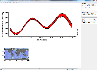
Instructions for Getting Started with Ocean Data View - How to Open ODV Spreadsheet Text Files
We recommend that users install the latest version of Ocean Data View from the ODV website. (Version 4 or newer is recommended for ARGO flag support). ODV's getting started guide can be found on their documentation page.
For an even faster start, follow these directions: start Ocean Data View, select File->Open, change the type of file to 'Data Files' so that it will find and accept .TXT files. To add more data to an existing collection (such as the one just created by opening a .TXT), select Import->ODV Spreadsheet. As data is added and plots are made, the data collection is automatically saved in an .ODV file and a sub-folder containing additional data. If you exit Ocean Data View, you can resume your data collection by opening that .ODV file. The default view is a world map, which isn't interesting. To add a simple plot, select View->Layout Templates->SCATTER WINDOW. Following these steps with the above example ODV spreadsheet file, you should see this:
In addition, right-click on the plot to change which variables are plotted and access the plots' properties. For multiple device deployments, go to View->Station Selection Criteria and select different cruise labels to see the data from different device deployments. To sort out QAQC flags, right-click on the plot and select Sample Selection Criteria and then highlight the flags to filter the data inclusively.
Oceans 3.0 API filter: extension=txt
MAT (Matlab data file)
MAT files (v7) can be opened using Mathworks Matlab 7.0 or later. These files are limited to a size of ~400 MB (depending on compression within the file, once loaded in MATLAB, the memory footprint will less than 1 GB). The file contains two structures, metadata and data.
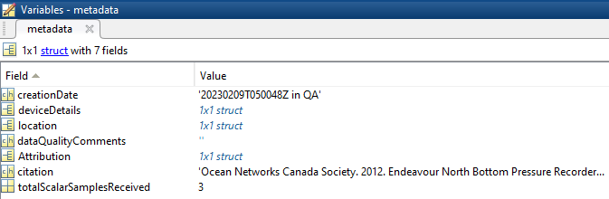
- creationDate:Date and time (using ISO8601 format) that the data product was produced. This is a valuable indicator for comparing to other revisions of the same data product.
- deviceDetails: a structure array with a structure for each deployment, with the following fields:
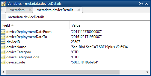
- deviceDeploymentDateFrom
- deviceDeploymentDateTo
- deviceID: A unique identifier to represent the instrument within the ONC observatory.
- deviceName: A name given to the instrument.
- deviceCategory: A unique name given to the category of devices, such as 'CTD'
- deviceCategoryCode: Code representing the device category. Used for accessing webservices, as described here: API / webservice documentation (log in to see this link).
- deviceCode: A unique string for the instrument which is used to generate instrument search data product file names.
- location: a structure array with a structure for each deployment location, with the following fields:
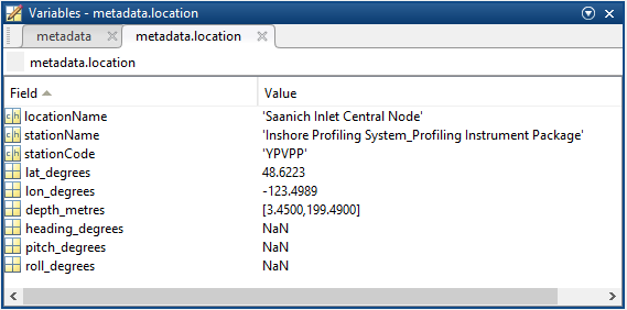
- stationName: Secondary location name.
- stationCode: Code representing the station. Used for accessing webservices, as described here: API / webservice documentation (log in to see this link).
- depth_metres: Obtained at time of deployment. If NaN, the device is mobile and this position is a variable, the data for which is supplied by a sensor in the data struct.
- lat_degrees: Obtained at time of deployment. If NaN, the device is mobile and this position is a variable, the data for which is supplied by a sensor in the data struct.
- lon_degrees: Obtained at time of deployment. If NaN, the device is mobile and this position is a variable, the data for which is supplied by a sensor in the data struct.
- heading_degrees: Obtained at time of deployment. If NaN, the device is mobile and this position is a variable, the data for which is supplied by a sensor in the data struct.
- pitch_degrees: Obtained at time of deployment. If NaN, the device is mobile and this position is a variable, the data for which is supplied by a sensor in the data struct.
- roll_degrees: Obtained at time of deployment. If NaN, the device is mobile and this position is a variable, the data for which is supplied by a sensor in the data struct.
- dataQualityComments: In some cases, there are particular quality-related issues that are mentioned here. This is distinct from QAQC information contained in the data structure.
- Attribution: A structure array with information on any contributors, ordered by importance and date. If an organization has more than one role it will be collated. If there are gaps in the date ranges, they are filled in with the default Ocean Networks Canada attribution (seen in example below). If the "Citation Required?" field is set to "No" on the Network Console then the citation will not appear. Here are the fields:
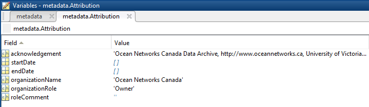
- acknowledgement: usually formatted as "<organizationName> (<organizationRole>)", except for when there are no attributions and the default is used (as shown above). This text is used to attribute plots when there are contributors other than ONC.
- startDate: datenum format
- endDate: datenum format
- organizationName
- organizationRole: comma separated list of roles
- roleComment: primarily for internal use, usually used to reference relevant parts of the data agreement (may not appear)
- citation: a char array containing the DOI citation text as it appears on the Dataset Landing Page. The citation text is formatted as follows: <Author(s) in alphabetical order>. <Publication Year>. <Title, consisting of Location Name (from searchTreeNodeName or siteName in ONC database) Deployed <Deployment Date (sitedevicedatefrom in ONC database)>. <Repository>. <Persistent Identifier, which is either a DOI URL or the queryPID (search_dtlid in ONC database)>. Accessed Date <query creation date (search.datecreated in ONC database)>
- totalScalarSamplesReceived: The number of time stamps that have any valid data on any sensor (at each time stamp). Only defined for metaData(1).totalScalarSamplesReceived, as this total is a summary of all device deployments in the data product.
data: a structure array (one structure per sensor) containing the following:
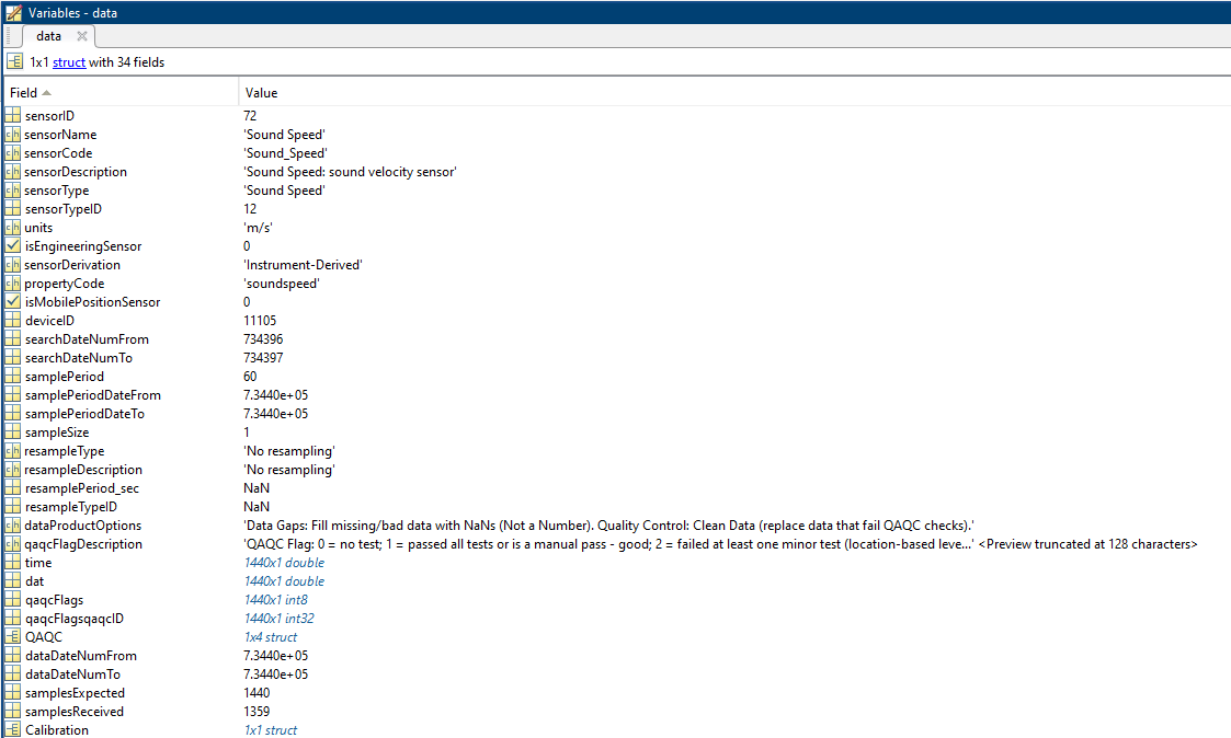
^ A single sensor, while as an array (multiple sensors / device-level), it looks like this: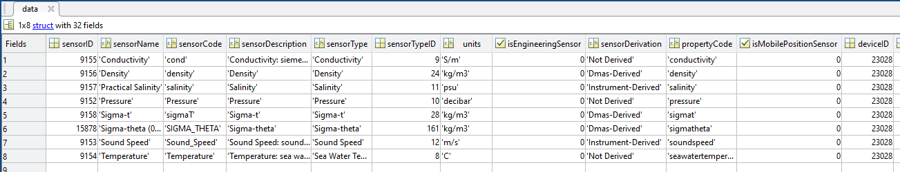
(screen grab cut off for width). The fields in the data structure are defined as:
- sensorID: Unique identifier number for each sensor (can be multiple for searches that combine data from multiple deployments)
sensorName: Name of sensor.
sensorCode: Unique string for the sensor.
sensorDescription: Description of sensor.
sensorType: Type of sensor as classified in the ONC data model.
sensorTypeID: ONC ID given to sensor type.
units: Unit of measure for the sensor data.
isEngineeringSensor: boolean (flag) to determine if sensor is an engineering sensor.
sensorDerivation: String describing the source of the sensor data: derived from calibration formula (dmas-derived), calculated on the device (instrument-derived), calculated by an external process (externally-derived), or direct from the instrument.
- propertyCode: unique string for the sensor that is used in the Oceans 3.0 API.
isMobilePositionSensor: boolean (flag) to determine if sensor is a mobile sensor. Note, this will only be flagged true if this data was added in addition to the requested data. For example, if the user requests a device-level mat product from a GPS device, then the latitude sensor is not flagged. Conversely, if the user requests temperature data from a mobile platform like a ship, then the latitude data from the GPS is added and interpolated to match the time stamps of the temperature sensor. See Positioning and Attitude for Mobile Devices for more information.
deviceID: Unique identifier number for the parent device.
searchDateNumFrom: Start date of the specific search in MATLAB datenum format - searches are truncated by availability and deployment dates.
searchDateNumTo: End date of the specific search MATLAB datenum format - searches are truncated by availability and deployment dates.
samplePeriod: Vector of sample periods in seconds (specific to this sensor, maybe different from other sensors and the device-level sample period).
samplePeriodDateFrom: Vector of the start date of each sample period/size (MATLAB datenum format).
samplePeriodDateTo: Vector of the end date of each of sample period/size (MATLAB datenum format).
sampleSize: The size of the data sample (specific to this sensor, maybe different from other sensors and the device-level sample size).
resampleType: Type of resampling used.
resampleDescription: Description of the resampleing used.
resamplePeriod_sec: Resample period in seconds.
resampleTypeID: Unique identifier of the subsample type used: 0/NaN - none, 1 - average, 2 - decimated (not offered), 3 - min/max, 4 - linear interpolation (VPS pressure only).
dataProductOptions: A string describing the data product options selected for this data product. This information is reflected in the file name.
qaqcFlagDescription: A string describing the flags. See the QAQC page for more information.
time: A vector of data timestamps in MATLAB datenum format.
- Available when not resampling and for resampling by average:
dat: A vector of sensor values corresponding to each timestamp. When resampling by averaging, this becomes the average value drawn from the resampling time window, also known as "box-car average" as documented here: Time Averaging and Resampling. (May make a separate field for this in the future, especially if users prefer that option).
qaqcFlags: A vector indicating the quality of the data, matching the time and dat vectors. See the QAQC page for more information. Note that this is the final, compiled/combined flag, the result of multiple automated tests and manual flags.
Available when not resampling:
- qaqcFlagsqaqcID: A vector containing the qaqcID of the QAQC test that contributed the final flag in the qaqcFlags vector above. The qaqcID corresponds to the tests & flags in the QAQC structure that is shown below. In the case of missing data (where the qaqcFlag is nine) and when there is no qaqc test (qaqcFlag is zero), qaqcFlagsqaqcID will have a value of zero. Mobile position sensors' data may carry qaqcFlagsqaqcID values through where there's no interpolation otherwise qaqcFlagsqaqcID will have a value of zero.
- Available when resampling by average or min/max + average only (not shown in the screenshot above):
- timeAverage: A vector of the mean value of the time stamps that populate each resampling time window.
- count: A vector with the number of samples within each resampling time window that contributes to the average value expressed in data.dat.
- standardDeviation: A vector of the sample standard deviation calculated from the data within each resampling time window.
- Available when min/max or min/max + avg resampling only (not shown in the screenshot above):
- dataMinimum & datMaximum: Vectors of min or max values from each resampling time window.
- countMinMax: A vector with the number of samples within each resampling time window that are available for min/max resampling (when min/max + avg resampling this can be different than the count for the average).
- timeMinimum & timeMaximum: Vectors of the time stamps at the min or max value within each resampling time window.
- qaqcFlagsMin & qaqcFlagsMax: Vectors of the qaqcFlags value at the min or max value within each resampling time window.
dataDateNumFrom: First time-stamp of the time series.
dataDateNumTo: Last time-stamp of the time series.
samplesExpected: The number of valid samples expected from the minimum returned data to the maximum returned data, accounting for variations in sample period.
samplesReceived: The number of raw samples received, maybe less than length(data.time) when data gaps are being filled with the NaN option.
Calibration: Structure (not pictured) containing information on the calibration formula applied to the data, as a it appears on the sensor listing page, in the JEP language. Fields include: dateFrom, dateTo, sensorID, name, formula.
QAQC: Structure containing all of the QAQC data for the time range of the search for the sensor. Each test and sensor combination will be a instance of this structure. Fields include: qaqcID, sensorID, dateFrom, dateTo, qaqcFlag, sourceSensorID, testLevel, priority, description. These field names are the same as found on the QAQC test definitions page: https://data.oceannetworks.ca/QaqcAutotestsFinder with additional fields priority and sourceSensorID, where priority is the priority level for flag combination that is defined by testLevel, while sourceSensorID is the sensorID on which the test was originally applied on. When sourceSensorID and sensorID are different, the test was inherited via a calibration formula; salinity is common example where it will inherit tests on conductivity and temperature. The test formula and attribute values are included as well (where applicable, manual flags do not have formulae), primarily for the benefit of internal users. The formulas are somewhat difficult to parse, Contact Support if you have questions. As a primer, x is the value under test, "$" indicates an internal variable that is available within the system (often mobile position sensor values like "$heading"), while the letter "A" followed by a three digit number, such as "A629", is an attribute contained in the TestAttributes structure where the three digit number is the attributeID. To see all the details of the test, such as the test attribute thresholds, use the aforementioned QaqcAutotestsFinder or go directly to the test definition page by using this URL: https://data.oceannetworks.ca/QaqcAutotestDetails?qaqcId=1, replacing the "1" with the QAQC.qaqcID of the test you wish to investigate. For internal users, please note that the qaqcFlag value is updated from it's value in the database (pass or fail) to it's nominal flag values (0,1,2,3,4) as defined in Quality Assurance Quality Control. For each time stamp (data.time), the final QAQC value (data.qaqcFlags) is determined by combining all of the flags that are applicable at that time. Averaging / resampling data further combines flags within the resample period. This process is documented here: Quality Assurance Quality Control. The final data.qaqcFlags value is then a somewhat complicated combination of tests and flags (essentially the worst flag wins trumped by the manual flag). The QAQC structure is provided to support users investigating final flag values, allowing one to trace backwards to the contributing tests. When not resampling, see data.qaqcFlagsqaqcID to see the qaqcID of the test that contributed the final flag values. Additionally, to see all the tests and test parameters that contributed to the final flag, pass the data.time value to the following blurb of code. It returns a subset of the QAQC structure that contains the tests that were applicable at the target time:
Here's an example of what the QAQC structure looks like in MATLAB (taken from the example MAT file below, salinity sensor shown to demonstrate inheritance):
Putting it all together, here's an example of the data.qaqcFlags, data.qaqcFlagsqaqcID vectors and data.QAQC structure next to each other, showing how users can simply scan through and see what tests are contributing to the final flag: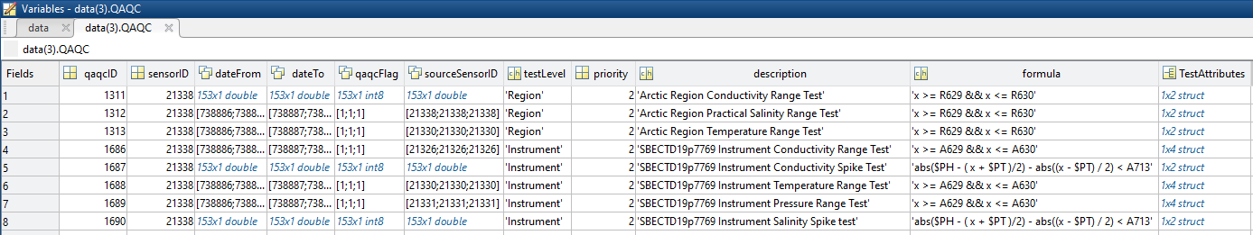
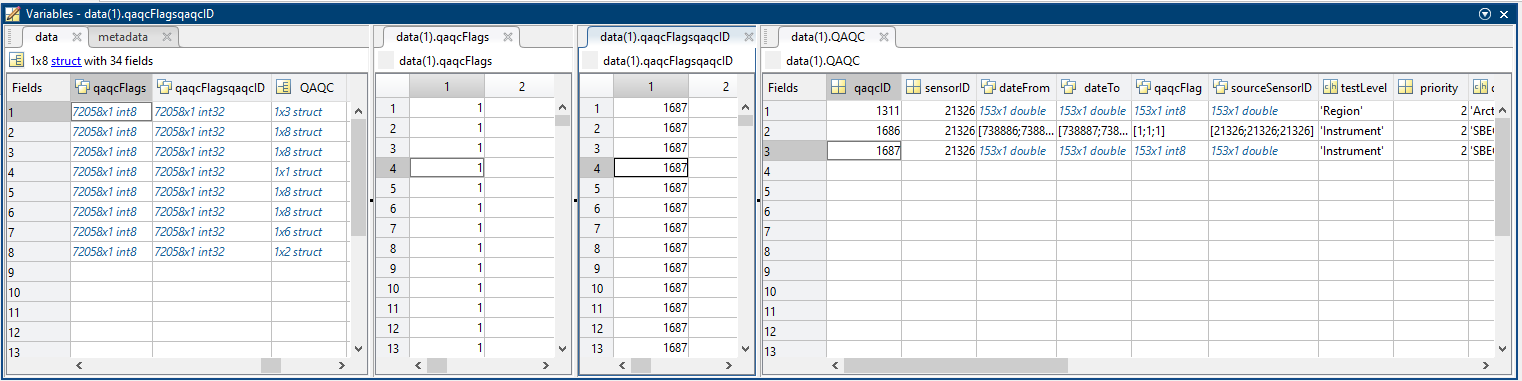
Note that products derived from the time series scalar MAT file will not have the QAQC structure and qaqcFlagsqaqcID vector. This currently includes, but is not limited to Thomson De-tided MAT files and the water column data products: 56 and 61. In general, this extra QAQC information is only relevant to original sample rate time series scalar data and is best handled by MAT files.
EXAMPLE FILE: CambridgeBay_UnderwaterNetwork_ConductivityTemperatureDepth_20230101T000000Z_20230101T235959Z-NaN_clean.mat
Oceans 3.0 API filter: extension=mat
NetCDF
NetCDF files are a common, widely used binary format, that is compact, efficient and can be self-describing, especially when used with data standards and conventions, as described here: NetCDF. ONC's time series scalar NetCDF format is very similar to the above MAT format. Fun fact, MAT files and NetCDF files use the same file format basis: HDF5 (MAT7 and NetCDF4). The data product is still in the prototype and internal development phase - specifically, the exact metadata content is still under development. Once this is tested and released, the layout and structure will be documented below. Please contact us if you need to access this format.
Oceans 3.0 API filter: extension=nc
Discussion
To comment on this product, click Write a comment... below.