ASL Acoustic Profiler Time Series
Data products for ASL Environmental Sciences echosounders are described here. Currently, three echosounder types are supported: the Zooplankton Acoustic Profiler (ZAP), the Acoustic Water Column Profiler (AWCP) and the Acoustic Zooplankton and Acoustic Zooplankton Fish Profiler (AZFP). The Shallow Water Ice Profiler (SWIP) is a similar instrument, however it only reports ice draft scalar data, not echosounder backscatter; SWIP data is available via scalar data products. Echosounder backscatter data is numerically intense, generating some of the largest data sets at ONC. Because of this, ASL echosounder data products for extended time ranges will be slow to generate and download. In addition, ASL echosounders produce ancillary scalar data, such as temperature, pitch, roll, which are available independently as scalar data products or via Plotting Utility.
ONC has worked closely with ASL Environmental Sciences, providing a testbed for the development of their echosounders, especially for their calibration. Users may notice that the ZAP is the simplest of the echosounders, while the AZFP is the most advanced. This is reflected in the MAT file product as MAT files from the ZAPs have a number of empty fields. In order to create a MAT file product that works with as many echosounders as possible, including multi-frequency AWCPs and AZFPs, the format and layout of the MAT file is more complex then the original ZAP mat file format available on the VENUS data download page. Users of ZAP data from the VENUS data download page will find more information on the more generic ASL MAT file format below, including a matlab script that can be used to convert MAT files into the VENUS ZAP format. The script is also useful as a guide for users to update their code to the new file format. Once updated, users can process ASL data from a combination of ZAP, AWCP and AZFP echosounder over a long time range, seamlessly. (ZAPs are slowly being phased out in favour of AZFPs.)
EchoView is a popular data analysis and visualization software for echosounders. There are two data product formats that EchoView can read: ASL EchoView export CSV and ASL's binary format .01a file, both of which are described below.
ASL manufacturer's documentation:
ZAP: AWCP:
AZFP:
(Note that these are static - newer versions maybe available and may not be updated here. Contact us or ASL for the latest documentation.)
AZFPlink and similar manufacturer's software for ZAP and AWCP is available from ASL, see their website: https://aslenv.com/azfp.html
For internal users, additional useful information, data, files, etc, maybe found in Alfresco: ASL device documentation.
Oceans 3.0 API filter: dataProductCode=AAPTS
Revision History
- 20110302: Beta MAT product released
- 20141028: Major revision: support AZFP and AWCPs, integrate options, process requests from all networks, improve performance, standardize MAT files, add plots
- 20150504: Major revision: add support for ZAPs, add sun elevation graph
- 20191204: Add ASL EchoView export format CSV files, add Target Strength calculation, add Noise Suppression option
- 20200107: Add ASL (manufacturer's) binary format .01a file (with xml configuration files for EchoView integration)
Data Product Options
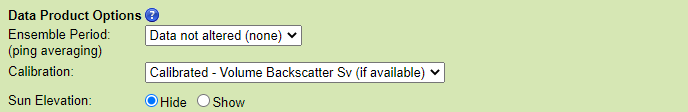
Ensemble Period (ping averaging)
This option will cause the search to perform the standard box-car average resampling on the data. 'Boxes' of time are defined based on the ensemble period, e.g. starting every 15 minutes on the 15s, with the time stamp given as the center of the 'box'. Acoustic pings that occur within that box are averaged range or bin-wise, and the summary statistics, such as 'Data.nPingsAcquired' (from ASL time series MAT files) are updated. This process is often called 'ping averaging'. The process uses log scale averaging, which involves backing out the dB scale to pressure, compute the weighted average, and then compute the dB scale again. Weighted averages are used when raw files bridge an ensemble period and when the data is already an ensemble or ping average.
New files are started when the maximum records per file is exceeded (files will not exceed 1 GB of memory when loaded), or when there is a configuration, device or site changes. In the case where there is data from either side of a configuration change within one ensemble period, two files will be produced with the same ensemble period, the same time stamps, but different data. Users may use the ensemble statistics on the number of pings or samples per ensemble to filter out ensembles that do not have enough data. (As an aside, we do this by default with clean averaged scalar data - each ensemble period needs to have at least 70% of it's expected data to be reported as good.)
For plotting data products, the requested ensemble period may be overridden to prevent image aliasing (one ensemble period is prevented from being smaller than one pixel). Also, the requested ensemble period also selects if the plots are broken daily (none option) or allowed to span multiple days (breaks still occur at configuration changes and internal data/memory limits).
The default value for this option is no averaging, meaning the data is not altered.
Some echosounders are configured to do ping averaging during acquisition, so the data you request with with 'Data not altered (none)' could already be averaged. To determine if the echosounder is averaging data as it is acquiring it, check the device details page (e.g. http://dmas.uvic.ca/DeviceListing?DeviceId=22608, go to the additional attributes tab) or check the data products: see the comment field in the plots or the Config structure in MAT files, look for Config.p in the ASL time series (BioSonics echosounder don't usually do any onboard averaging). Available ensemble periods are 0.5, 1, 5, 10, 15 and 60 minutes.
Data not altered
Oceans 3.0 API filter:
dpo_ensemblePeriod=030 Seconds
Oceans 3.0 API filter:
dpo_ensemblePeriod=201 Minute
Oceans 3.0 API filter:
dpo_ensemblePeriod=605 Minute
Oceans 3.0 API filter:
dpo_ensemblePeriod=30010 Minute
Oceans 3.0 API filter:
dpo_ensemblePeriod=60015 Minute
Oceans 3.0 API filter:
dpo_ensemblePeriod=9001 Hour
Oceans 3.0 API filter:
dpo_ensemblePeriod=3600
File-name mode field
Selecting an ensemble period will add 'Ensemble' followed by the ensemble period. For example '-Ensemble600s'.
Calibration
This option will apply the calibration to the data, when the calibration coefficients are available. The calibration calculation and coefficients are supplied by the manufacturer. See the device details page (additional attributes tab) to see the coefficients, see the instrument documentation page, or contact us for more details. These values are also provided in the MAT file products; see the Config / Cal structure for ASL data products and the data.snd.rxee structure for BioSonics data products.
The default value is to apply calibration and calculate the Volume Backscatter when available. Users may also choose a Target Strength calculation for calibrated data The former is used to estimate bio-mass of schools or aggregations, with the latter is useful with single large targets such as predatory fish (for more information see the format descriptions). The uncalibrated option will provide the raw data only. Raw data has units of raw counts, which are proportional to the received acoustic pressure.
Calibrated - Volume Backscatter Sv (if available)
Oceans 3.0 API filter:
dpo_calibration=1Calibrated - Target Strength TS (if available)
Oceans 3.0 API filter:
dpo_calibration=2Uncalibrated (raw pressure)
Oceans 3.0 API filter:
dpo_calibration=0
File-name mode field
'CalibratedSv' or 'CalibratedTS' will be added if all the channels of the device were successfully calibrated (for Volume Backscatter or Target Strength, respectively).
Sun Elevation
This option applies to echosounder plots only. If 'Show' is selected, it appends a graph of the Sun's elevation over time below the acoustic data, such a plot is useful to correlate the acoustic data with dial (daily) and tidal effects, such as zooplankton migrations.
The default will not add a plot of sun elevation.
Hide
Oceans 3.0 API filter:
dpo_sunElevation=0Show
Oceans 3.0 API filter:
dpo_sunElevation=1
File-name mode field
No affect on file-name.
Backscatter Colour Map
For Nortek and RDI ADCP daily current plot products (PNG and PDF formats) and echosounder backscatter plots (ASL, BioSonics)
This option allows the user to select the colourmap used for the backscatter plot. An example of each colourmap available is displayed below, along with the Oceans 3.0 API filter for that specific colourmap.
Default (ONC/VENUS rainbow/jet colours)
Oceans 3.0 API filter:
dpo_backScatterColourmap=0
Modified Default (perceptually smooth rainbow/jet colours from m_map toolbox)
Oceans 3.0 API filter:
dpo_backScatterColourmap=1
Sourced from: Pawlowicz, R., 2019. "M_Map: A mapping package for MATLAB", version 1.4k, [Computer software], available online at www.eoas.ubc.ca/~rich/map.html.
Sequential Blue to Purple (perceptually balanced - from colorbrewer.org)
Oceans 3.0 API filter:
dpo_backScatterColourmap=2
Sourced from: Charles (2020). cbrewer : colorbrewer schemes for Matlab (https://www.mathworks.com/matlabcentral/fileexchange/34087-cbrewer-colorbrewer-schemes-for-matlab), MATLAB Central File Exchange. Retrieved January 7, 2020.
Sequential Red to Yellow (perceptually balanced - from colorbrewer.org)
Oceans 3.0 API filter: dpo_backScatterColourmap=3

Sourced from: Charles (2020). cbrewer : colorbrewer schemes for Matlab (https://www.mathworks.com/matlabcentral/fileexchange/34087-cbrewer-colorbrewer-schemes-for-matlab), MATLAB Central File Exchange. Retrieved January 7, 2020.
Sequential Blue to Yellow (perceptually balanced - MATLAB Parula)
Oceans 3.0 API filter:
dpo_backScatterColourmap=4
Diverging Spectral (perceptually balanced - from colorbrewer.org)
Oceans 3.0 API filter:
dpo_backScatterColourmap=5
Sourced from: Charles (2020). cbrewer : colorbrewer schemes for Matlab (https://www.mathworks.com/matlabcentral/fileexchange/34087-cbrewer-colorbrewer-schemes-for-matlab), MATLAB Central File Exchange. Retrieved January 7, 2020.
Echosounder Noise Suppression
Applies to ASL data products.

This option only applies to the ASL Zooplankton Acoustic Profiler (ZAP) echosounder, but does appear as option for all ASL echosounders (due to a limitation on how we can display the option). It will have no effect on echosounders other than the ASL ZAP. An ONC-customized noise suppression algorithm is applied to the ZAP data by default, this option allows the user to switch it off and reproduce ASL's standard processing of the data.
On
Oceans 3.0 API filter:
dpo_zapNoiseSuppression=1Off
Oceans 3.0 API filter:
dpo_zapNoiseSuppression=0
Applies to ASL .01a Binary Data Files only.

This option allows users to choose the source to emulate for the binary files. In the normal raw file acquisition process for ASL echosounders, users can copy the files directly off of the Compact FLASH drive and this format is compatible with EchoView data analysis and visualization software. This is the default option. Alternatively, the Unaltered Serial Stream data is available, this is the data that ONC drivers record in real-time: Big-Endian with packet headers, as if one were recording the RS232 communications directly. Compared to the Serial Stream, the Compact FLASH format is also Big-Endian, but the packet headers are replaced with FLAG. Another format that is not offered is called 'Real-time' data: these are .001 files acquired via the ASL software (via RS232 serial communications), but stripped of packet headers and converted to Little-Endian; this source could be added at a future date, upon request.
- Emulate reading from Compact FLASH
Oceans 3.0 API filter:
dpo_aslBinarySource=0 - Unaltered Serial Stream
Oceans 3.0 API filter:
dpo_aslBinarySource=1
File-name mode field
The non-default, Unaltered Serial Stream option adds '-SerialStream' file mode modifier.
Formats
Processed data is available in MAT, CSV, PNG and PDF formats. The manufacturer's raw binary format, 01A, is also available. It replicates the nominal way of acquiring data from autonomous / stand-alone devices. Both it and the CSV file format can be loaded into popular visualization software EchoView (link). The CSV format replicates ASL's data export from their software, with options for Volume Backscatter and Target Strength output. The MAT, PNG and PDF file/plots (respectively) are general purpose and also have the same options as the CSV export format. Further content descriptions and examples are provided below.
When a driver/device restart is detected, the configuration is checked and if the configuration changed, all data products will break and a new file will be started (configuration breaks are also noted in the search status and logs). For all non-averaged data products and daily plots, a new file is started at the start of each day (in addition to configuration breaks). For ensemble-averaged MAT/CSV files and multi-day plots, the files can extend over multiple days, while file breaks will still occur for configuration changes and if the files get too big (MAT/CSV files will break if they occupy more than 1 GB of memory).
Calibrated data are represented in Volume Backscatter strength in units of dB re 1 m-1 or in Target Strength in units of dB re 1 m2. Without calibration, the data is in units of raw counts which is proportional to the pressure amplitude. When plotting raw data, the data is still plotted in a dB scale relative to the full scale of the device, where 0 dB represents the maximum value, normally 65535 raw counts for 16 bit data, and the lowest value is the 20*log10 value of the smallest value the A/D converter will produce (about -48 dB for ZAPs, about -96 dB for AWCPs and about -120 dB for AZFPs). Details on the calibration algorithm and formulae can be found here: https://support.echoview.com/WebHelp/Reference/Algorithms/Echosounder/ASL/AZFP_Sv_and_TS.htm (hard copy here: EchoViewManual_AZFP_Sv_and_TS.pdf).
For multi-frequency echosounders with separately mounted transducers, we account for the height variances with the device attribute Echosounder_TransducerHeight, which is utilized in both the plots and presented in the Meta structure in the MAT files.
Data files: MAT
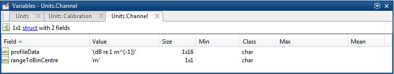
MAT files (v7) can be opened using MathWorks MATLAB 7.0 or later. The file contains four structures: Meta, Data, Config, and Units. The structures are the same for AWCP, AZFP or ZAP ASL echosounders. Data Search / Oceans 3.0 ZAP MAT files can be converted to the VENUS ZAP format (no longer available) by a conversion script that is provided below. Screenshots below capture what the MAT file will look like loaded in MATLAB's workspace.
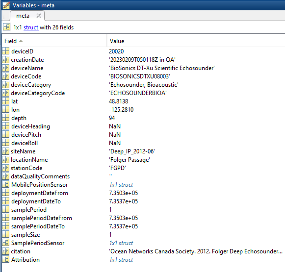
- deviceID: A unique identifier to represent the instrument within the Ocean Networks Canada data management and archiving system.
- creationDate:Date and time (using ISO8601 format) that the data product was produced. This is a valuable indicator for comparing to other revisions of the same data product.
- deviceName: A name given to the instrument.
- deviceCode: A unique string for the instrument which is used to generate data product filenames.
- deviceCategory: Device category to list under data search ('Echosounder').
- deviceCategoryCode: Code representing the device category. Used for accessing webservices, as described here: API / webservice documentation (log in to see this link).
- lat: Fixed value obtained at time of deployment. Will be NaN if mobile or if both site latitude and device offset are null. If mobile, sensor information will be available in mobilePositionSensor structure..
- lon: Fixed value obtained at time of deployment. Will be NaN if mobile or if both site longitude and device offset are null. If mobile, sensor information will be available in mobilePositionSensor structure.
- depth: Fixed value obtained at time of deployment. Will be NaN if mobile or if both site depth and device offset are null. If mobile, sensor information will be available in mobilePositionSensor structure.
- deviceHeading: Fixed value obtained at time of deployment. Will be NaN if mobile or if both site heading and device offset are null. If mobile, sensor information will be available in mobilePositionSensor structure.
- devicePitch: Fixed value obtained at time of deployment. Will be NaN if mobile or if both site pitch and device offset are null. If mobile, sensor information will be available in mobilePositionSensor structure.
- deviceRoll: Fixed value obtained at time of deployment. Will be NaN if mobile or if both site roll and device offset are null. If mobile, sensor information will be available in mobilePositionSensor structure.
- siteName: Name corresponding to its latitude, longitude, depth position.
- locationName: The node of the Ocean Networks Canada observatory. Each location contains many sites.
- stationCode: Code representing the station or site. Used for accessing webservices, as described here: API / webservice documentation (log in to see this link).
- dataQualityComments: In some cases, there are particular quality-related issues that are mentioned here.
- MobilePositionSensor: A structure with information about sensors that provide additional scalar data on positioning and attitude (latitude, longitidue, depth below sea surface, heading, pitch, yaw, etc).
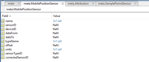
- name: A cell array of sensor names for mobile position sensors. If not a mobile device, this will be an empty cell string.
- sensorID: An array of unique identifiers of sensors that provide position data for mobile devices - this data may be used in this data product.
- deviceID: An array of unique identifiers of devices that provide position data for mobile devices - this data may be used in this data product.
- dateFrom: An array of datenums denoting the range of applicability of each mobile position sensor - this data may be used in this data product.
- dateTo: An array of datenums denoting the range of applicability of each mobile position sensor - this data may be used in this data product.
- typeName: A cell array of sensor names for mobile position sensors. If not a mobile device, this will be an empty cell string. One of: Latitude, Longitude, Depth, COMPASS_SENSOR, Pitch, Roll.
- offset: An array of offsets between the mobile position sensors' values and the position of the device (for instance, if cabled profiler has a depth sensor that is 1.2 m above the device, the offset will be -1.2m).
- sensorTypeID: An array of unique identifiers for the sensor type.
- correctedSensorID: An array of unique identifiers of sensors that provide corrected mobile positioning data. This is generally used for profiling deployments where the latency is corrected for: CTD casts primarily.
- deploymentDateFrom: The date of the deployment on which the data was acquired.
- deploymentDateTo: The date of the end of the deployment on which the data was acquired (will be NaN if still deployed).
- samplingPeriod: Sample period / data rating of the device in seconds, this is the sample period that controls the polling or reporting rate of the device (some parsed scalar sensors may report faster, some devices report in bursts) (may be omitted for some data products).
- samplingPeriodDateFrom: matlab datenum of the start of the corresponding sample period (may be omitted for some data products).
- samplingPeriodDateTo: matlab datenum of the end of the corresponding sample period (may be omitted for some data products).
- sampleSize: the number of readings per sample period, normally 1, except for instruments that report in bursts. Will be zero for intermittent devices (may be omitted for some data products).
- SamplePeriodSensor: A structure array with an entry for each scalar sensor on the device (even though this metadata is for complex data products that don't use scalar sensors).
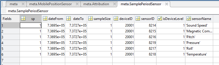
- sp: sample period in seconds (array), unless sensorid is NaN then this is the device sample period
- dateFrom: array of date from / start date (inclusive) for each sample period in MATLAB datenum format.
- dateTo: array of date to / end date (exclusive) for each sample period in MATLAB datenum format.
- sampleSize: the number of readings per sample period (array). Normally 1, except for instruments that report in bursts. Will be zero for intermittent devices.
- deviceID: array of unique identifiers of devices (should all be the same).
- sensorID: array of unique identifiers of sensors on this device.
- isDeviceLevel: flag (logical) that indicates, when true or 1, if the corresponding sample period/size is from the device-level information (i.e. applies to all sensors and the device driver's poll rate).
- sensorName: the name of the sensor for which the sample period/size applies (much more user friendly than a sensorID).
- citation: a char array containing the DOI citation text as it appears on the Dataset Landing Page. The citation text is formatted as follows: <Author(s) in alphabetical order>. <Publication Year>. <Title, consisting of Location Name (from searchTreeNodeName or siteName in ONC database) Deployed <Deployment Date (sitedevicedatefrom in ONC database)>. <Repository>. <Persistent Identifier, which is either a DOI URL or the queryPID (search_dtlid in ONC database)>. Accessed Date <query creation date (search.datecreated in ONC database)>
- Attribution: A structure array with information on any contributors, ordered by importance and date. If an organization has more than one role it will be collated. If there are gaps in the date ranges, they are filled in with the default Ocean Networks Canada citation. If the "Attribution Required?" field is set to "No" on the Network Console then the citation will not appear. Here are the fields:
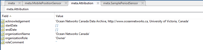
- acknowledgement: the acknowledgement text, usually formatted as "<organizationName> (<organizationRole>)", except for when there are no attributions and the default is used (as shown above).
- startDate: datenum format
- endDate: datenum format
- organizationName
- organizationRole: comma separated list of roles
- roleComment: primarily for internal use, usually used to reference relevant parts of the data agreement (may not appear)
Not shown above:
Meta.transducerHeight - This is an offset height (m) relative to the instruments' base level, used to account for the varying heights of multi-frequency, separately mounted tranducers. By ONC convention the site depth is the depth the instrument platform floor, while the siteDevice offset is the depth change from the platform to the instrument, but in this case that offset will be measured to the transducer mounting base.
It should be noted that if a multi-channel device is sporadically missing pings in some but not all channels, in the MAT format these gaps in the data will be filled with NaN values to adhere to common indexing between the channels, whereas the raw 01A file format will skip that channel's missing ping altogether. This will appear as a discrepancy between these two file types.
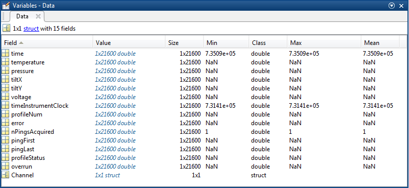
Data: structure containing the AWCP data, having the following fields. Everything outside of the Channel structure applies to all channels.
- time: vector, timestamp in datenum format (obtained from time the reading reached the shore station, or if the ping averaging option was selected, these time stamps will be resampled).
- temperature: vector, temperature time-series (will be filled with NaNs if not available). Calibration formula:
vin = tempRawCounts * 2.5 / 65535;
R = (ka + kb * vin) / (kc - vin);
temperature = (1/(A + B * log(R) + C * (log(R)^3))) - 272.15; - pressure: vector, pressure time-series (will be filled with NaNs if not available). Note: calibration not yet available, these sensors are not calibrated or even connected, do not use this data.
- tiltX: vector, tilt X-direction time-series (will be filled with NaNs if not available). Calibration formula:
X_a * txc + X_b * txc + X_c * txc + X_d, where txc is the raw tilt counts in the x direction - tiltY: vector, tilt Y-direction time-series (will be filled with NaNs if not available). Calibration formula:
Y_a * txc + Y_b * txc + Y_c * txc + Y_d, where txc is the raw tilt counts in the x direction - voltage: vector, battery voltage time-series (will be filled with NaNs if not available)
- timeInstrumentClock: vector, instrument clock time-series
- ProfileNum: vector, profile number
- error: vector, error code
- nPingsAquired: vector, number of pings acquired for profile
- pingFirst: vector, index of first ping acquired in profile
- pingLast: vector, index of last ping acquired in profile
- profileStatus: vector, profile status code
- overrun: vector, (we think) this indicates if the data hit the limit of the A/D converter.
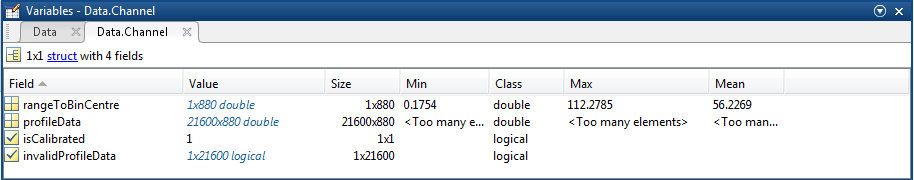
- Channel: structure (one for each channel, so access is by Data.channel(3) for example), with the following fields:
- rangeToBinCentre: vector of length of the number of bins. The range to the centre of each bin is calculated from two-way travel time, accounting for sound speed, lockout distance and one half of the pulse length.
- profileData: 2D matrix (time, rangeToBinCentre) of the acoustic data. The acoustic data can be raw counts from the echosounder's Analogue to Digital converter (A/D), or if calibrated, it will be Volume Backscatter or Target Strength data in units of dB re 1 m-1 or dB re 1 m2 (respectively). See the Unit structure or the isCalibrated flag (below) in order to tell the two apart. Here is the calibration formula applied to convert raw profile data to calibrated profile Volume Backscatter (Sv) data for AWCPs and AZFPs:
N = (log10(Data.Channel(i).profileData) - 2.5) * 524280 * Config.Calibration.DS(i);
Data.Channel(i).profileData = Config.Calibration.EL(i) - 2.5/Config.Calibration.DS(i) + ...
N/(26214*Config.Calibration.DS(i)) - Config.Calibration.TVR(i) - 20*log10(Config.Calibration.VTX0(i)) + 20*log10(R) + ...
2*Config.Calibration.acousticAttenuation(i) * R - ...
10*log10( (1/2) * Config.speedOfSound * (Config.pulseLength(i)*1e-6) * Config.Calibration.BP(i) );
Here is the calibration formula for ZAPs:Data.Channel(i).profileData = -Config.Calibration.OCV(i) - Config.Calibration.sourceLevel(i) - 20*log10(Config.Calibration.Q(i)) + 20*log10(R) +...
2*Config.Calibration.acousticAttenuation(i) * R -...
10*log10( (1/2) * Config.speedOfSound * (Config.pulseLength(i)*1e-6) * Config.Calibration.BP(i) ) +...
20*log10(Data.Channel(i).profileData) - repmat(Config.Calibration.zapInterpTVG(i,:), size(Data.Channel(i).profileData, 1), 1);
where i is the channel number and R is the rangeToBinCentre (replicated into a matrix). The calibration procedure also accounts for the gain and time-varying-gain applied. In the case of the ZAP echosounder, an optional noise reduction algorithm is also applied (contact us or more details). To calculate the Target Strength (TS, units of dB re 1 m2,) the 20logR term becomes 40logR and the ensonification term is dropped (the term with the beampattern BP and pulse length), as detailed here: EchoViewManual_AZFP_Sv_and_TS.pdf
- rawData: 2D matrix (time, rangeToBinCentre) of the acoustic data. When non-calibrated data is requested for ZAP echosounders only, this matrix is provided as the most raw data. In that case, profileData represents the noise-reduced raw data (contact us for more details).
- isCalibrated: integer, 0 indicates the data is not calibration, 1 indicates volume backscatter data in units of dB re 1 m-1, 2 indicates Target Strength in units of dB re 1 m2. Calibration may be requested but no provided if not available. This flag represents what the data is, not what was requested.
- invalidProfileData: logical vector, custom added field by our code that indicates if the raw data was truncated before the expected number of range bins was returned. Invalid data are filled with NaNs. We have seen partial data in truncated pings, which could be extracted, however, this data does not appear to be reliable. If you wish to see this data, contact us and we can provide it.
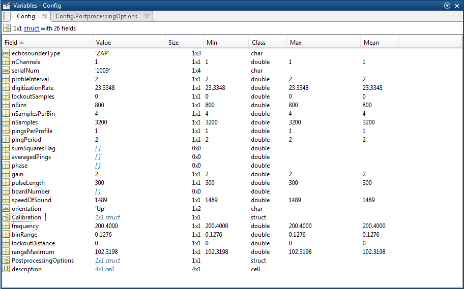
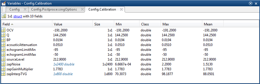
Config: structure containing instrument configuration details. For details about the configuration parameters, refer to the manufacturer documentation. This structure contains a conglomeration of parameters from all 3 types. All parameters are the original instrument settings as read from the raw data except otherwise noted (in particular, Calibration, speedOfSpeed, orientation and ProcessingOptions are applied in postprocessing to calibrate the data)
- echosounderType: string, name of the echosounder type (used on the plot).
- nChannels: number of channels (in case instrument is capable of having multiple frequencies)
- serialNum: serial number of device
- profileInterval: number of seconds per profile (or burst interval, reflects onboard ensemble averaging for AWCP / AZFP, otherwise equal to data rating or ping interval)
- digitizationRate: rate at which received signal is digitized, per channel
- lockoutSamples: number of samples to ignore
- nBins: number of bins in profile, per channel
- nSamplesPerBin: number of samples used to calculate amplitude in each bin, per channel. This is known as Range Averaging. For AZFPs and AWCPs, this is a configurable parameter, for ZAPs it was fixed.
- nSamples: number of samples in profile, per channel. This is the number of raw samples: nBins * nSamplesPerBin or maxRange * digitizationRange * 2 / speedOfSound, where maxRange is not the same as rangeMaximum below, but is max(Data.Channel(1).rangeToBinCentre) + binRange/2
- pingsPerProfle: number of pings to average for profile, per channel (onboard ensemble averaging only)
- pingPeriod: number of seconds between pings
- sumSquaresFlag: flag to indicate if sum of squares values calculated onboard AWCPs only and included in the raw data (onboard ensemble averaging only)
- averagedPings: flag to indicate if averaging was done onboard AZFPs only (onboard ensemble averaging only, probably replaced the sumSquaresFlag)
- phase: phase used to acquire profile (AWCP/AZFP only, not used in any processing or display)
- gain: gain setting, per channel (affects time-varying-gain on AWCP and ZAP)
- pulseLength: pulse length, per channel
- boardNumber: board number, per channel
These values may not be read from the raw data:
- speedOfSpeed: sound speed used for calculation of range (single value determined from median conditions in the water column for device's deployment location, in units of m/s), used in post-processing.
- orientation: 'Up' is the normal case for all echosounders mounted on the seabed, facing up towards the sea surface, while 'Down' is the case for echosounders mounted on ships, buoys, etc. We use this flag for plotting purposes. The y-axis in the time-series 'echogram' plots will be calculated as follows: for 'Up': binDepth = Meta.depth - Data.channel.rangeToBinCentre, for 'Down': binDepth = Meta.depth - Data.channel.rangeToBinCentre, unless Meta.depth is NaN. In that case, we plot the echosounder's range as the y-axis. (Meta.Depth == NaN means the echosounder is mobile. In the future we may produce a plot that accounts for mobile echosounders.) (Available late November, 2014.)
- Calibration: structure containing calibration data stored in device attributes. For AZFP and AWCPs, these values originate from configuration text (.cfg) files that ship with the instruments. For ZAPs, these values originate from ONC calibration reports. See the instrument documentation pages for more details, we can also provide the formulas by which these values are applied. The Calibration structure includes:
- tilt sensor calibration coefficients (fields starting with X or Y)
- pressure sensor calibration co-efficients (fields starting with k, plus A, B, C)
- backscatter calibration parameters, fields: TVR, VTX0, EL, DS, BP, AcousticAttenuation (attenuation is a single value determined from median conditions in water column for device's deployment location, in units of dB/m). For ZAP: OCV, Q, sourceLevel, zapInterpTVG, zapNoise, zapGainMultiplier
- frequency: frequency of echosounder, per channel (AWCP/AZFP read from data, ZAP stored attribute)
- binRange: two-way distance spanned by each bin (calculated from digitizationRate, speedOfSpeed, pulseLength)
- lockoutDistance: blanking distance (based on number of lockout samples), per channel
- rangeMaximum: maximum range from which samples are digitized, per channel. This is useful to indicate the last or furthest possible contribution to the data, which is distinct from the maximum value of Data.channel.rangeToBinCentre. For rangeMaximum, the value is calculated as the number of bins times the bin range, plus the pulse duration times sound speed divided by 2; in other words, to the end of the last bin and to the end of transmit pulse.
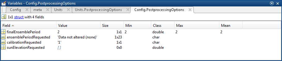
- PostprocessingOptions: structure containing the post-processing options
- finalEnsemblePeriod: final ensemble period. For non-averaged mat files, this will be Config.profileInterval, for plots and averaged mat files, this is the final ensemble averaging period
- ensemblePeriodRequested: ensemble averaging option selected by the user
- calibrationRequested: calibration averaging option select by the user, calibration may not be available, see Data.Channel.isCalibrated. 1 for yes, 0 for no
- sunElevationRequested: show the sun elevation graph? 1 for yes, 0 for no (for plotting products only, for MAT files, this will be empty)
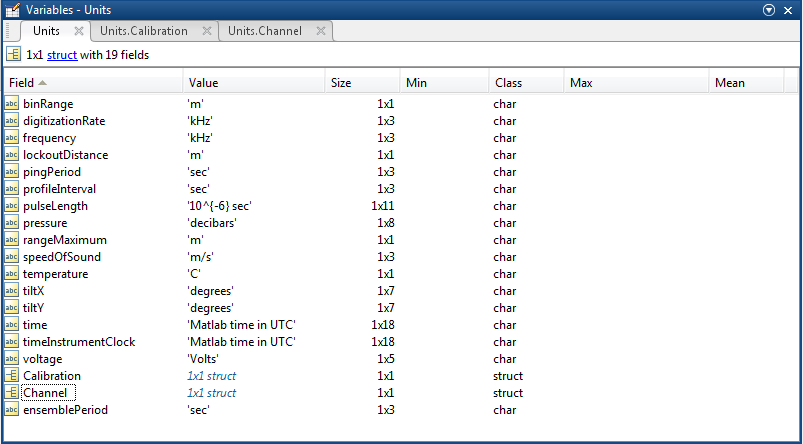
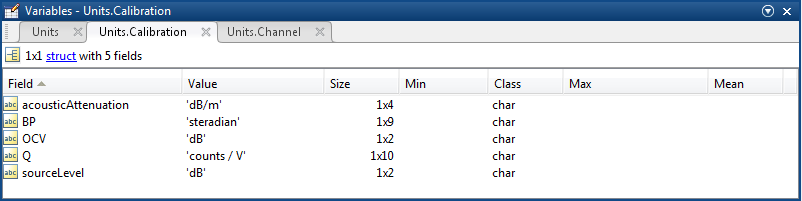
Units: structure containing unit of measure for fields in structures above. For instance, units.frequency='kHz'. Note that channel specfic data units: profileData, rangeToBinCentre are stored in Units.channel(1).
Oceans 3.0 API filter: extension=mat
ASL Profiler Time Series MAT file Conversion Script
This script will convert MAT files to the VENUS ZAP MAT file format. It works on data loaded in the workspace and is intended to be used as basis for users to adapt their code and analysis to the new format, which will be the standard format into the future. Download the script file and open in matlab, press the 'run' button, the script will open a window to select an ASL Profiler MAT file to process, after loading the ASL Profiler MAT file, the workspace will be populated with the familar ZAP MAT file structures: zapdata, config, units, meta, while the ASL MAT file structures will remain (ASL MAT file structures follow the MATLAB convention of naming structures with upper case letters).

ASL export CSV files
In the ASL software (AZFPLink in the case of AZFPs), there is an option to export a CSV data file of the Volume Backscatter and/or Target Strength profiles. This data product replicates that export. The resulting files contain the same data as the above MAT file product., conforming to the export format that is compatible with EchoView's import. If users export with the calibrated option on, they can view the data directly in EchoView without the need for further information. AZFPLink does also export a binary representation of this file with the header and ancillary information in a CSV file and the backscatter in a simple binary file named with the extension .bin. This .bin format is not available. We find that the full CSV file is the same size when compressed and works just as well.
Here is an example of the CSV files, one file for each of the backscatter or target strength, pitch and roll:
Ping_date,Ping_time,Ping_milliseconds,Range_start,Range_stop,Sample_count
2010-07-15,17:07:30,000,3.974,303.6045,310,15158.7879,43856.4848,38595.8788,43027.3939,37114.1818,34455.7576,37149.0909,31756.1212,33549.5758,35378.9091,33622.7879,32621.0909,33328.9697,34967.7576,35500.1212,34936.7273,35635.3939,36515.3939,36298.1818,37105.9394,38320.0000,39600.0000,38311.7576,38841.6970,40223.5152,39821.5758,40156.1212,41004.1212,42024.2424,42155.1515,42266.6667,43222.7879,43354.1818,43892.8485,44316.1212,45424.0000,45287.7576,46349.0909,46881.9394,47687.7576,47800.2424,48639.0303,50095.0303,49871.5152,50920.7273,51827.3939,53208.7273,52925.0909,53704.2424,55041.9394,55893.8182,56475.1515,57305.2121,58848.4848,59510.7879,59648.0000,60767.0303,62110.5455,62964.8485,63652.8485,64165.5152,21828.8788,1001.7273,1766.3333,2651.1818,4319.0606,4646.8182,5064.2727,6559.5455,7796.8788,8751.5455,9614.0909,10852.8788,11745.4848,12020.8788,12798.5758,14140.6364,14782.5758,16420.3939,16761.2424,18595.9091,18881.0000,20056.2727,21441.4848,22530.4545,23694.5758,23746.9394,25738.6970,26960.5152,27918.0909,28682.2121,29971.9091,30910.5758,32291.4242,34234.2121,35137.0000,35608.7576,37312.5152,38407.3030,40157.6061,40645.3636,42447.5455,44778.6970,46330.6970,46746.2121,48523.6667,50326.8182,52144.5152,52448.5152,55404.6364,56951.7879,58677.3636,60197.3636,62435.4242,63222.0000,54947.7576,13899.6970,3776.0606,5030.8485,7386.2424,10165.3939,10981.8788,12804.4242,14163.4545,17818.2424,18387.4545,19278.1212,22337.0303,24881.5152,26477.1515,27950.1212,30141.1515,32853.8788,33106.0000,35080.7879,37490.9697,40905.7576,41193.7576,43433.2727,46501.8788,47261.6364,50346.2424,51242.2424,53858.4848,56198.3636,57398.8485,60814.1212,62876.8182,53708.8485,22199.3636,2770.5152,5088.0909,7382.8788,10037.9091,11289.7879,15374.1515,18600.8182,19863.8485,24318.6364,23879.3636,25360.5758,29742.6364,32305.0606,33809.0606,36128.5758,41094.3939,43251.9697,44568.8182,48982.3939,53572.4545,56884.4545,58250.2727,62643.1818,23153.4242,12894.1818,6220.2424,8491.2727,14916.9697,17185.0909,22244.0000,23924.0000,27132.7273,31124.4848,35360.1212,39689.8182,41905.5758,45684.4848,50564.4848,54799.1515,57115.7576,59601.5758,33729.6061,4327.1212,25141.9697,8949.0000,14878.2121,16875.3030,19733.0000,24058.3333,29793.6061,31581.7273,35933.7273,39416.3939,46422.9394,45410.0909,50831.6667,54343.9091,59280.7879,53033.8485,34345.6970,18739.0909,10117.0303,10285.2727,15842.1212,22682.3636,25281.1515,27929.8788,35333.0303,40794.3636,43626.8485,48743.4545,53628.3030,59328.1818,33870.0909,15316.8788,22547.6061,14462.2727,20772.5758,27896.9394,36022.0303,39263.2424,41160.4545,53256.4545,56267.6970,40652.3333,35656.4848,10201.4545,18168.4848,21519.2727,27829.0909,44085.5758,41553.2121,48818.3333,49756.8485,35393.5455,20159.7879,13866.4545,25146.4545,30530.2121,35267.6667,43849.4848,53850.6061,49871.0000,22332.7576,15675.4545,15968.7879,17430.1212,28082.7273,44135.0909,50059.9394,53342.5152,48185.3636,16466.0909,23662.3939,20307.2424,27098.5152,38341.1818,38198.1515,49617.1212,42732.7879,15190.8182,27358.9091,19465.0909,34849.8182,38096.3636,39147.0303,56421.6970,33140.1212,21738.5758,16621.0000,30931.7879,39198.9394,46495.9091,57656.1818,3301.7576,19685.7576,22773.7576,30513.8788,46854.7273,52101.9394,46775.4242,20342.2727,7870.0303,13266.3939,19263.9697,25435.6061,31347.8485,31905.4242,37936.9394,42724.8182,44331.6061,48077.5455,51512.2121,55631.0000,56692.3333,62028.0909,65535.0000,65535.0000,65535.0000,65535.0000
2010-07-15,17:22:30,000,3.974,303.6045,310,15154.6667,43898.6667,38562.6667,43026.6667,37109.3333,34485.3333,37184.0000,31776.0000,33525.3333,35365.3333,33653.3333,32632.0000,33346.6667,34981.3333,35488.0000,34978.6667,35626.6667,36509.3333,36346.6667,37149.3333,38282.6667,39570.6667,38290.6667,38888.0000,40181.3333,39866.6667,40186.6667,41048.0000,42093.3333,42192.0000,42288.0000,43242.6667,43373.3333,43890.6667,44322.6667,45416.0000,45298.6667,46365.3333,46941.3333,47714.6667,47845.3333,48666.6667,50096.0000,49898.6667,50952.0000,51848.0000,53261.3333,52893.3333,53706.6667,55061.3333,55936.0000,56469.3333,57320.0000,58829.3333,59520.0000,59632.0000,60760.0000,62184.0000,62976.0000,63669.3333,64206.0000,21817.0000,1017.0000,1793.0000,2681.0000,4323.6667,4606.3333,5038.3333,6619.6667,7862.3333,8739.6667,9606.3333,10859.6667,11731.6667,12030.3333,12803.6667,14150.3333,14721.0000,16433.0000,16763.6667,18598.3333,18883.6667,20091.6667,21465.0000,22571.6667,23638.3333,23798.3333,25726.3333,26921.0000,27889.0000,28721.0000,29878.3333,30870.3333,32273.0000,34185.0000,35150.3333,35598.3333,37342.3333,38401.0000,40131.6667,40670.3333,42491.6667,44758.3333,46299.6667,46734.3333,48518.3333,50366.3333,52161.0000,52411.6667,55499.6667,56883.6667,58657.0000,60163.6667,62486.3333,63198.5000,53991.1667,12956.6667,3770.0000,5028.6667,7420.6667,10202.0000,10940.6667,12692.6667,14250.0000,17855.3333,18436.6667,19250.0000,22354.0000,24940.6667,26498.0000,27887.3333,30183.3333,32874.0000,33138.0000,35162.0000,37463.3333,40924.6667,41196.6667,43476.6667,46626.0000,47386.0000,50247.3333,51322.0000,53927.3333,56156.6667,57474.0000,60818.0000,62924.8333,52698.6667,22136.3333,2837.6667,5117.6667,7432.3333,10016.3333,11253.6667,15307.0000,18637.6667,19861.6667,24411.0000,23824.3333,25435.0000,29685.6667,32285.6667,33805.6667,36117.6667,41093.6667,43232.3333,44496.3333,49035.0000,53472.3333,56736.3333,58317.6667,62614.3333,23163.8333,13812.0000,6225.3333,8476.0000,14897.3333,17060.0000,22342.6667,23828.0000,27169.3333,31044.0000,35457.3333,39593.3333,41990.6667,45694.6667,50630.6667,54657.3333,56910.6667,59577.8333,32807.6667,4290.0000,26727.6667,8989.0000,14826.3333,16994.3333,19738.3333,24159.6667,29714.3333,31429.0000,35834.3333,39466.3333,46359.6667,45333.0000,50997.0000,54274.3333,59255.8333,52048.1667,33389.8333,18032.6667,10094.0000,10078.0000,16078.0000,22798.0000,25475.3333,28003.3333,35550.0000,40768.6667,43590.0000,49147.3333,53656.6667,59390.5000,32878.8333,14516.1667,21804.3333,14265.6667,21031.0000,28108.3333,36263.0000,39305.6667,41249.6667,53604.3333,56412.6667,40762.1667,34837.3333,10437.3333,18456.0000,21677.3333,28104.0000,44408.0000,41813.3333,48736.1667,48840.5000,34598.1667,19491.6667,13961.0000,25547.6667,30769.0000,35102.3333,44606.3333,53902.5000,48980.3333,22567.1667,16495.3333,15660.6667,17100.6667,27876.6667,44284.6667,50143.3333,53284.8333,47693.5000,15637.5000,22669.6667,19797.6667,27427.0000,38736.3333,38403.0000,49312.6667,41105.1667,14353.0000,27110.6667,19513.3333,34940.0000,37881.3333,38721.3333,56839.1667,32020.8333,22565.0000,16103.6667,30794.3333,39343.6667,46082.3333,57499.3333,3358.0000,19459.3333,22030.0000,30411.3333,46894.0000,51960.8333,47254.6667,22116.3333,7679.0000,12631.0000,18639.0000,25220.3333,30908.3333,31695.0000,37505.6667,42623.0000,44140.3333,47969.6667,51455.0000,55399.0000,56569.6667,61764.3333,65535.0000,65535.0000,65535.0000,65535.0000
2010-07-15,17:37:30,000,3.974,303.6045,310,15154.6667,43898.6667,38562.6667,43026.6667,37109.3333,34485.3333,37184.0000,31776.0000,33525.3333,35365.3333,33653.3333,32632.0000,33346.6667,34981.3333,35488.0000,34978.6667,35626.6667,36509.3333,36346.6667,37149.3333,38282.6667,39570.6667,38290.6667,38888.0000,40181.3333,39866.6667,40186.6667,41048.0000,42093.3333,42192.0000,42288.0000,43242.6667,43373.3333,43890.6667,44322.6667,45416.0000,45298.6667,46365.3333,46941.3333,47714.6667,47845.3333,48666.6667,50096.0000,49898.6667,50952.0000,51848.0000,53261.3333,52893.3333,53706.6667,55061.3333,55936.0000,56469.3333,57320.0000,58829.3333,59520.0000,59632.0000,60760.0000,62184.0000,62976.0000,63669.3333,64206.0000,21817.0000,1017.0000,1793.0000,2681.0000,4323.6667,4606.3333,5038.3333,6619.6667,7862.3333,8739.6667,9606.3333,10859.6667,11731.6667,12030.3333,12803.6667,14150.3333,14721.0000,16433.0000,16763.6667,18598.3333,18883.6667,20091.6667,21465.0000,22571.6667,23638.3333,23798.3333,25726.3333,26921.0000,27889.0000,28721.0000,29878.3333,30870.3333,32273.0000,34185.0000,35150.3333,35598.3333,37342.3333,38401.0000,40131.6667,40670.3333,42491.6667,44758.3333,46299.6667,46734.3333,48518.3333,50366.3333,52161.0000,52411.6667,55499.6667,56883.6667,58657.0000,60163.6667,62486.3333,63198.5000,53991.1667,12956.6667,3770.0000,5028.6667,7420.6667,10202.0000,10940.6667,12692.6667,14250.0000,17855.3333,18436.6667,19250.0000,22354.0000,24940.6667,26498.0000,27887.3333,30183.3333,32874.0000,33138.0000,35162.0000,37463.3333,40924.6667,41196.6667,43476.6667,46626.0000,47386.0000,50247.3333,51322.0000,53927.3333,56156.6667,57474.0000,60818.0000,62924.8333,52698.6667,22136.3333,2837.6667,5117.6667,7432.3333,10016.3333,11253.6667,15307.0000,18637.6667,19861.6667,24411.0000,23824.3333,25435.0000,29685.6667,32285.6667,33805.6667,36117.6667,41093.6667,43232.3333,44496.3333,49035.0000,53472.3333,56736.3333,58317.6667,62614.3333,23163.8333,13812.0000,6225.3333,8476.0000,14897.3333,17060.0000,22342.6667,23828.0000,27169.3333,31044.0000,35457.3333,39593.3333,41990.6667,45694.6667,50630.6667,54657.3333,56910.6667,59577.8333,32807.6667,4290.0000,26727.6667,8989.0000,14826.3333,16994.3333,19738.3333,24159.6667,29714.3333,31429.0000,35834.3333,39466.3333,46359.6667,45333.0000,50997.0000,54274.3333,59255.8333,52048.1667,33389.8333,18032.6667,10094.0000,10078.0000,16078.0000,22798.0000,25475.3333,28003.3333,35550.0000,40768.6667,43590.0000,49147.3333,53656.6667,59390.5000,32878.8333,14516.1667,21804.3333,14265.6667,21031.0000,28108.3333,36263.0000,39305.6667,41249.6667,53604.3333,56412.6667,40762.1667,34837.3333,10437.3333,18456.0000,21677.3333,28104.0000,44408.0000,41813.3333,48736.1667,48840.5000,34598.1667,19491.6667,13961.0000,25547.6667,30769.0000,35102.3333,44606.3333,53902.5000,48980.3333,22567.1667,16495.3333,15660.6667,17100.6667,27876.6667,44284.6667,50143.3333,53284.8333,47693.5000,15637.5000,22669.6667,19797.6667,27427.0000,38736.3333,38403.0000,49312.6667,41105.1667,14353.0000,27110.6667,19513.3333,34940.0000,37881.3333,38721.3333,56839.1667,32020.8333,22565.0000,16103.6667,30794.3333,39343.6667,46082.3333,57499.3333,3358.0000,19459.3333,22030.0000,30411.3333,46894.0000,51960.8333,47254.6667,22116.3333,7679.0000,12631.0000,18639.0000,25220.3333,30908.3333,31695.0000,37505.6667,42623.0000,44140.3333,47969.6667,51455.0000,55399.0000,56569.6667,61764.3333,65535.0000,65535.0000,65535.0000,65535.0000
The file-name modifiers include ensemble averaging, the string '-EchoView' (to avoid any possible confusion with other CSV products), the echosounder channel centre frequency and data type: (one of) pitch, roll, sv (Volume Backscatter), ts (Target Strength), raw (uncalibrated).
Oceans 3.0 API filter: extension=csv
ASL .01a raw binary data files
.01a files are the echosounder's binary raw internal data that is stored on the Compact Flash drive. In the normal raw file acquisition process for ASL echosounders, users usually copy the files directly off of the Compact FLASH drive. This format is compatible with a number of data analysis and visualization software, particularly EchoView (version 7.1 and later of EchoView will read .01a files). This is the default data product option. An alternate format, with the same file extension (.01a) is also available, denoted as Unaltered Serial Stream data. This is the data that ONC device drivers record in real-time: Big-Endian with packet headers, as if one were recording the RS232 communications directly. The is the "Real Time Profile Output Format" documented in Section 8.1 of the AZFP software manual. Compared to the Serial Stream, the Compact FLASH format is also Big-Endian, but the packet headers are replaced with a FLAG value, so that the file is FLAG-profile-FLAG-profile, etc, refer to Section 8.3 of the AZFP software manual for the Compact FLASH format. Another format that is not offered at this time is called 'Real Time Data Files' (section 8.4 in the manual): these are .001 files acquired via the ASL software (via RS232 serial communications), but with packet headers replaced with a different FLAG and converted to Little-Endian; this source could be added at a future date, upon request. The three variations also are documented in the AWCP user manual (posted at the top of this page), while the ZAP manual only documents the Serial Stream format (Appendix F in that manual).
The .01a files for AZFP and AWCP produced by the Compact FLASH option are readable by ASL's software (AZFPLink and their own MATLAB code) and a growing number of 3rd party software and code. See ASL's processing page https://aslenv.com/azfp-processing.html for more information. .01a files for ZAP echosounders produced by the Compact FLASH option are not likely to be readable however. Refer to Appendix F in WCP manual UVIC Venus version CM-100-WCP-01-R01.pdf - the profiles is taken from byte 27 (the ping interval) onward, excluding the last two byte (line feed, carriage return). Returning the entire packet with the Serial Stream option is likely to be the more usable option.
ONC's normal raw log files record all communication and data with the device in an ASCII hexadecimal format. This data product converts that hexidecimal data to binary, omitting driver commands and ASCII serial responses. The Serial Stream option is that direct output, whereas the Compact FLASH option has the addition trimming and insertions as noted. Live data is available for both options (the log files do not need to be archived for this data product to be available). Files are broken on the hour, every hour, with additional file breaks on driver restarts and configuration changes. On these configuration change breaks, the last letter in the file extension is incremented: .01a → .01b → .01c.
Accompanying these files will be .xml configuration metadata files, which are produced with the start of the data and for every configuration change. The format of the XML files is taken from the a recent ASL XML file, produced by AZFPLink version 1.0.30. AWCPs and earlier AZFPs generated a different XML file, while ZAP echosounders had a .cfg file (very similar to an XML file). The .xml file produced for all three echosounders is the AZFPLink version 1.0.30 format, with a few ONC comments to make it clear it wasn't produced by AZFPLink. The differences between all three are largely superficial - the XML tags for the calibration parameters are the same between the AZFP and AWCP echosounders, while the ZAP uses a formula and parameter set for calibration (see the calibration formulas detailed above). Here is an example ONC produced ASL .xml file: ASLAZFP55036_20140911T060000.742Z.xml (Newer versions of this file have a dateTo in the file-name).
A readMe text file accompanies the Compact FLASH format .01a files that aimed at helping EchoView load the data into EchoView, here is the content of that file (with added illustrations):
Dear Ocean Networks Canada data user,
This file contains additional instructions for users who wish to load and process our ASL manufacturer's binary format .01a files in EchoView.
All data products have extensive documentation. In this case, please refer to:
https://wiki.oceannetworks.ca/display/DP/24 (The section on .01a files is near the bottom of the page.)
We have learned of a few issues that EchoView users may encounter. (Thanks to our awesome users for their feedback.) These issues are:
* Confusion with the Data Search ISO-19115 metadata XML file. If the metadata XML file is in the same directory as the configuration XML files,
EchoView may attempt to load the metadata XML file, which of course contains no configuration information. Loading will succeed but users will
only see a default configuration in EchoView. How to fix: delete any files with names ending in META.xml from the directory containing the .01a files,
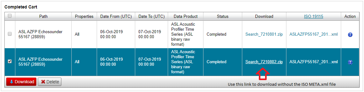
delete/clear EchoView to start over, import the .01a files again. How to avoid: when downloading data products from Data Search, users can skip
downloading the META.xml files by clicking on the data product link for each search, instead of the red download button that downloads all
products in a search cart, including the META.xml files. (We do recommend that users keep the META.xml files for reference, perhaps in
a separate directory.)
* EchoView may load the wrong configuration XML file if there are multiple configuration XML files in the directory where the user is loading
.01a files from. How to fix: check the directory where the data products have been unzipped after downloading. If there are multiple configuration
XML files, move each into separate directories. For each configuration, match the .01a files with the configuration XML files based on the time in
their filenames and move the .01a files to the directory with their corresponding configuration XML files.
* EchoView doesn't appear to reload XML files when new files are imported to an existing configuration. How to fix: always start with a
new project, load files grouped by their configuration as noted above.
* An alternative method is also offered: in Data Search, the CSV option under "ASL Acoustic Profiler Time Series" provides data files reproducing
the ASL software (AZFPLink) CSV export. These CSV files are calibrated (see the accompanying data product options) and are readily loaded into
EchoView. The disadvantages of this method include the lack of metadata that EchoView may need to perform other analysis, and that the file sizes
are quite large.
* EchoView has capabilities to manually input and edit configuration values, see their extensive and very useful help pages for this information.
* If all else fails, contact us: https://www.oceannetworks.ca/contact-us and/or contact EchoView customer support.
Enjoy,
- ONC Data Products and Data teams

We seek feedback on this data product. It is difficult to test and evaluate. Hopefully it is compatible with your software and uses. Please contact us if you need any support or would like to suggest changes.
Oceans 3.0 API filter: extension=01a
Plots: PNG and PDF
There are two formats of plots available: PNG or PDF. A PDF plot file can contain multiple plots as separate pages, and the graphics are vector images, which are better for printing or viewing at high resolution. The PNG format is a single plot per file in a raster image which is good for quick viewing and sharing. The data and appearance of the two plot formats are the same. These plots are also known as echograms, they plot echo intensity (backscatter, target strength or raw counts) vs time and depth, and are basically what you would see as a sonar operator. The calibration data product option switches the values plotted between raw (uncalibrated), Volume Backscatter (Sv) and Target Strength (TS), but does not otherwise affect the form and function of the plots. The plots are affected by the ensemble/averaging option, the number of channels, the deployment type (fixed vs. mobile) and the sun elevation data product option. As for all formats, plots always break on configuration changes. If plots extend over gaps in the data, users will see the gaps represented by white space.
Oceans 3.0 API filter: extension={png,pdf}
Plots: Daily vs Multi-day plots
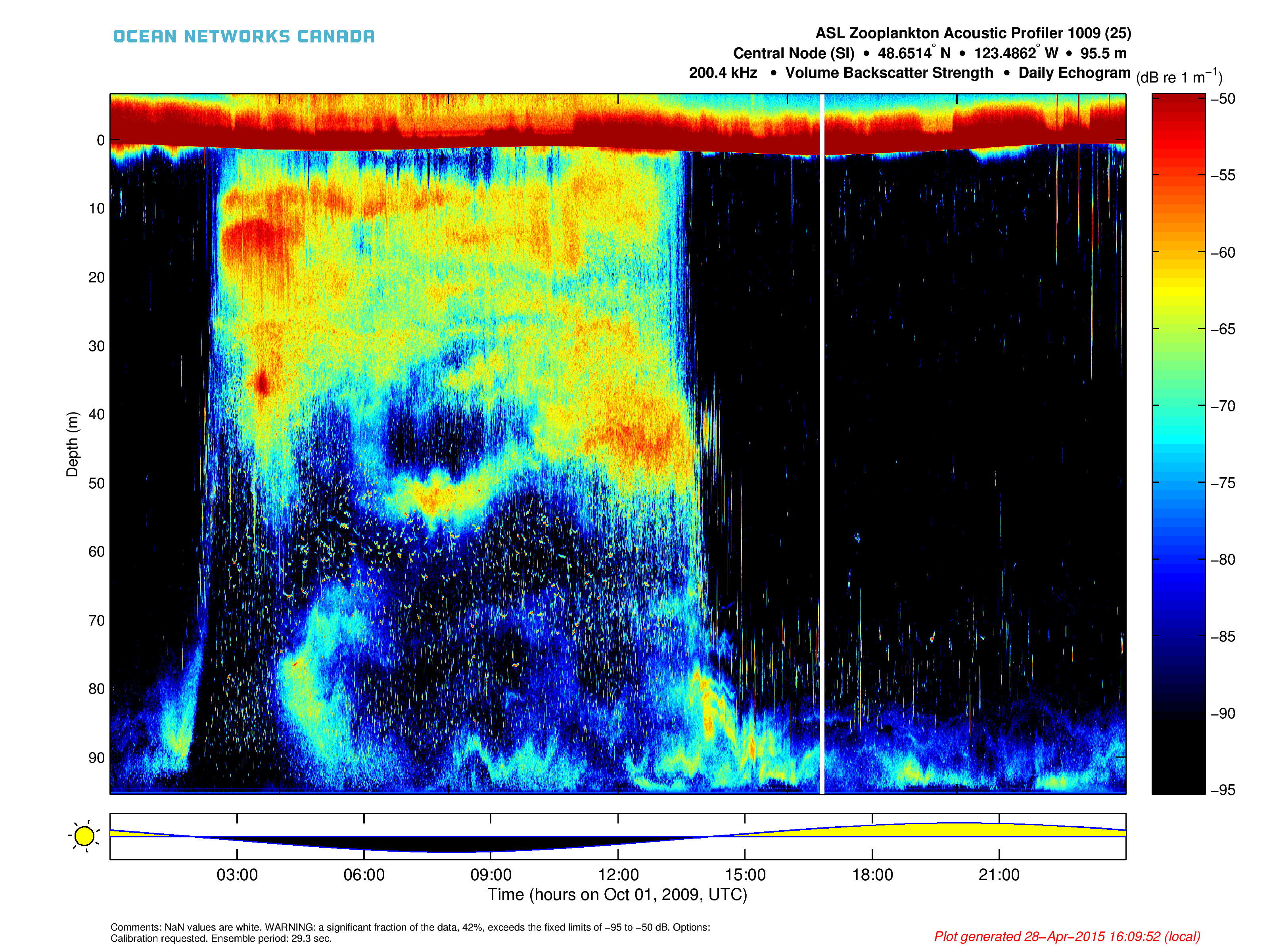
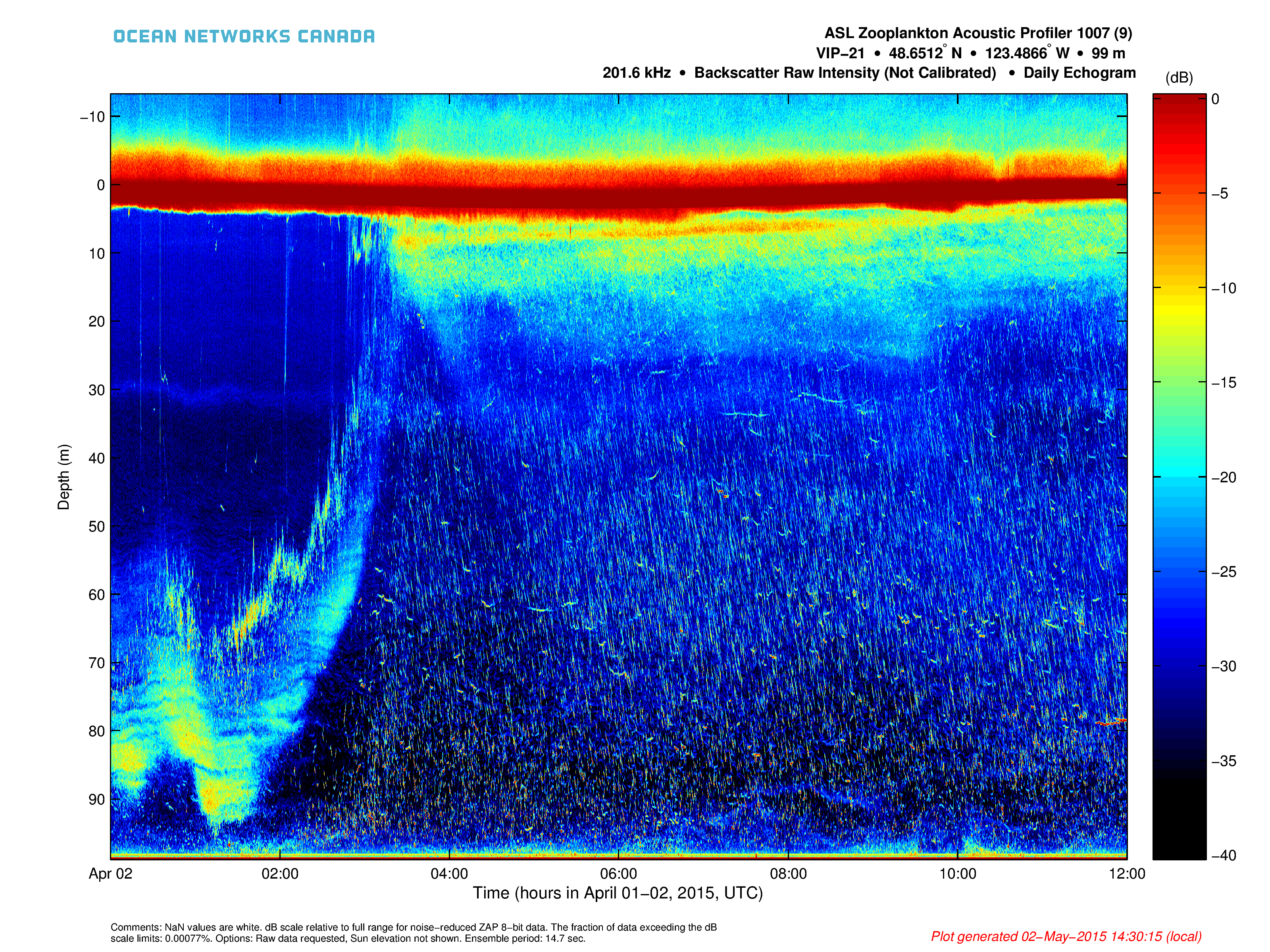
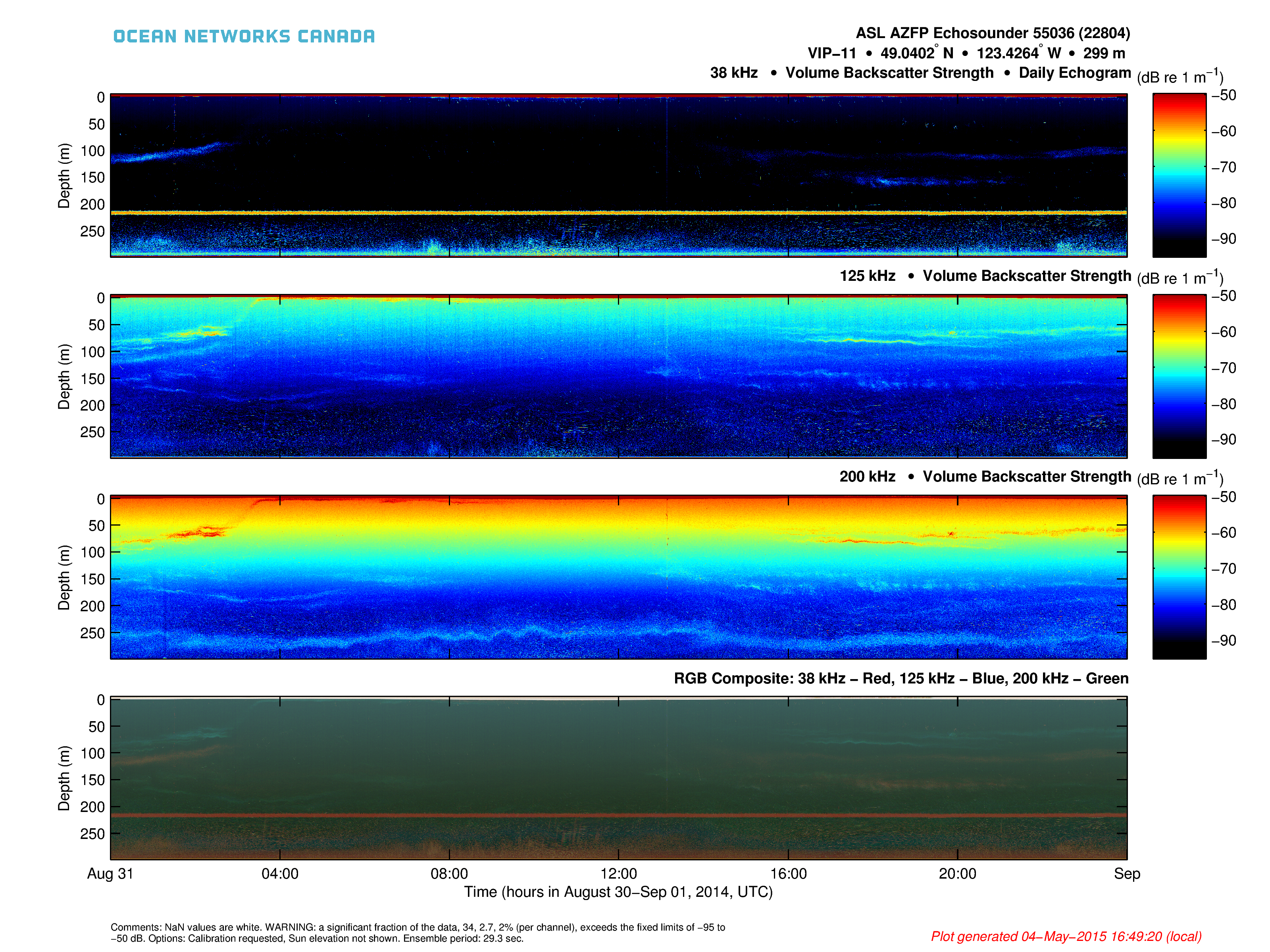
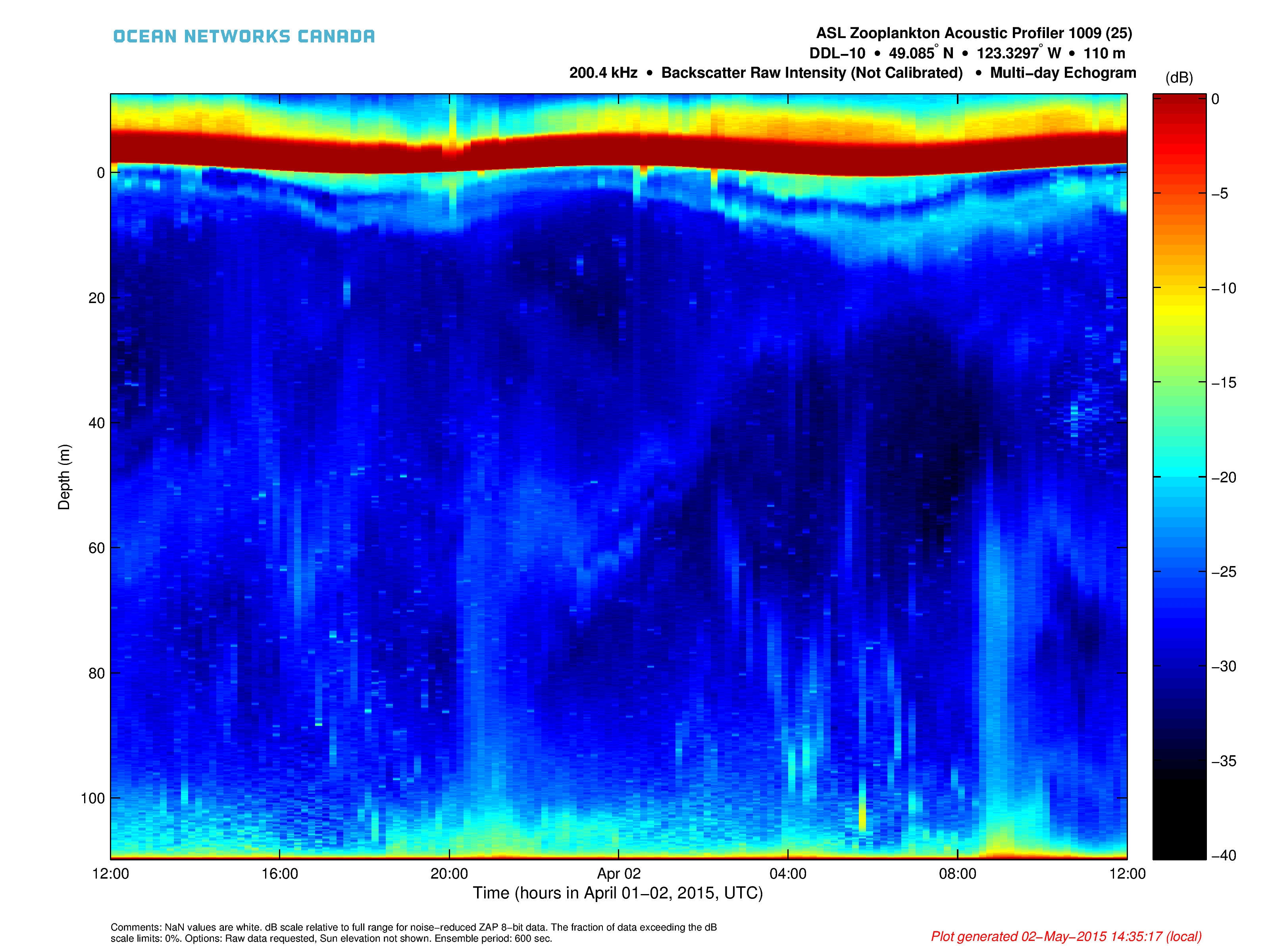
There are two variations of plots in terms of duration, depending on the ensemble period option selected. Daily plots are generated with the default (no averaging) option. Daily plots will show a maximum of one day of data per plot. For all plots, the data has to be resampled so that an ensemble or raw ping corresponds to the width of at least one pixel in the PNG (ideally one to one), otherwise rendering the image will alias the data; so in spite of selecting the no-averaging option, some resampling may happen. This resampling is important as normal resizing on computer screens applies linear image anti-aliasing routines which are not appropriate for logarithmic scale images. The minimum ensemble period for a one day plot is ~30 seconds as we have about 2560 pixels along the time axis in these plots. If you select less than one day, you can effectively zoom in and see higher temporal resolutions. Here are some examples of daily plots: first is a ZAP calibrated daily echogram with the sun elevation plot; second is a ZAP daily echogram, non-calibrated without the sun elevation plot, with a configuration change part way through the day; third is an AZFP calibration daily echogram without the sun elevation plot.
If an ensemble period is selected by the user (other than the none option), the plots will be multi-day plots and only one plot will be generated over the search time range (excluding configuration changes and data/memory limits, which break the plot). Ensemble averaging will be applied as selected, except when the selected ensemble period is not high enough to prevent aliasing and distortion, in which case the ensemble period will be increased automatically. Below are examples of multi-day plots from a ZAP and an AZFP with ensemble averaging set to 10 minutes, which is easily long enough to avoid aliasing and distortion.
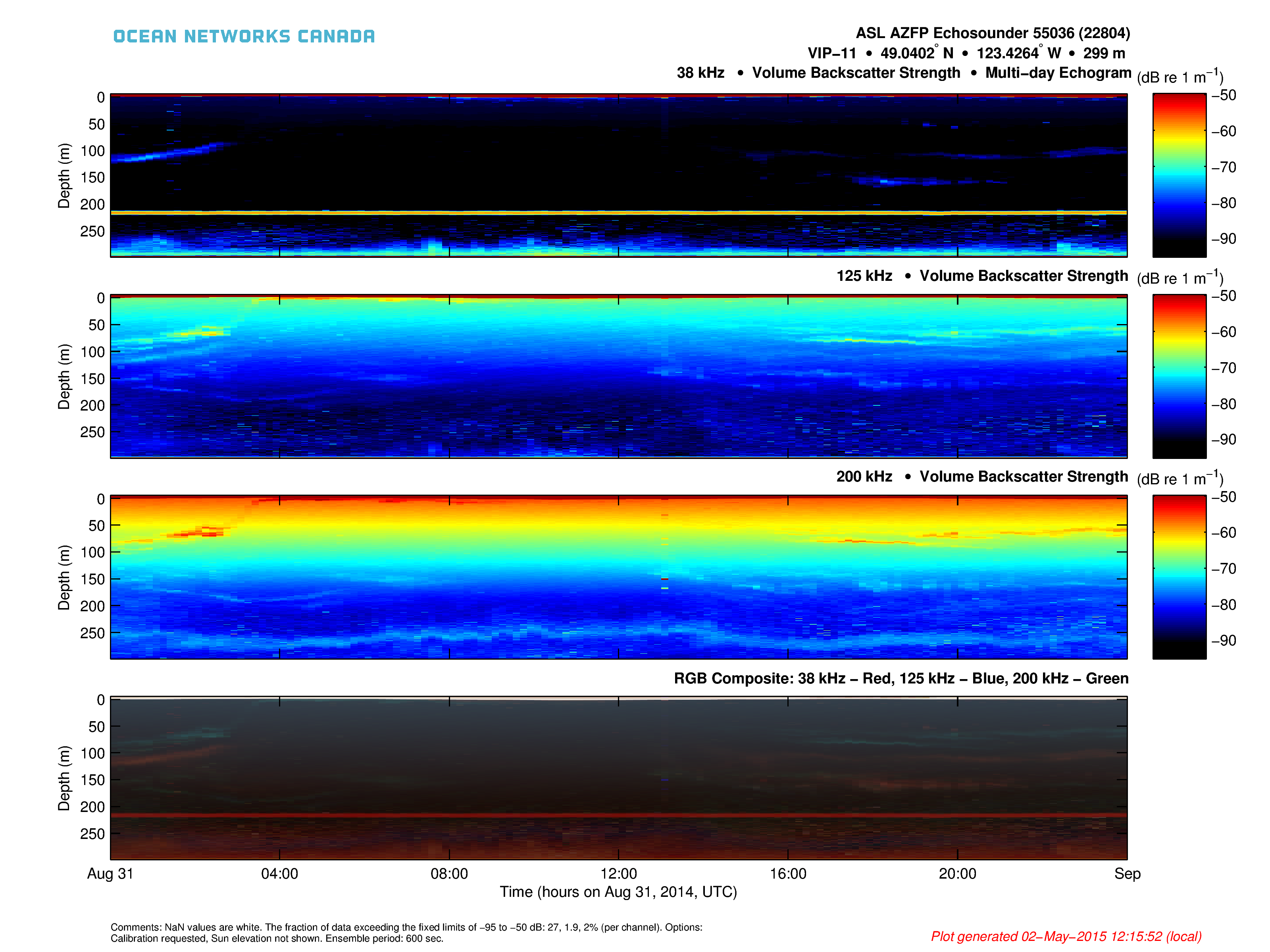
Plots: Single vs. Multiple Channels
If the echosounder has multiple channels, as in the examples above, each channel will be plotted as a subplot, with independent axis and limits. (Axis limits are set from fixed intervals, e.g. every 20 dB, to facilitate inter-plot comparison.) In addition, if the device has precisely 3 channels, an additional RGB composite plot will be shown. For the RGB subplot, each channel's data is represented by a primary colour, and the colours are combined to form an image. In this way, users can see composite details: various targets will appear as different colours, depending on their relative target strength as a function of frequency. This is useful for differentiating the targets between fish, zooplankton, bubbles, whales, etc.
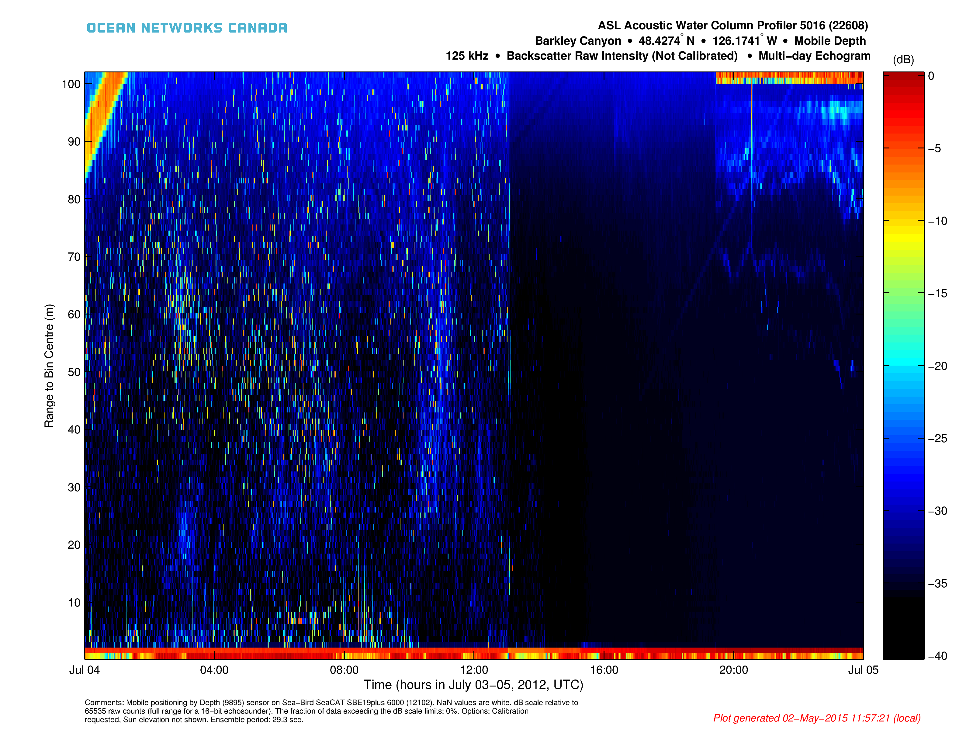
Plots: Mobile Depth
Here is an example of single channel plot, from a mobile AWCP echosounder on the vertical profile system where the y axis is not depth, but is instead echosounder range. We can't use depth as it is varying throughout the data. Future improvements maybe to register the pings with the varying depth, so that the y axis can be depth.
Discussion
To comment on this product, click Add Comment below.