Nortek Profiler Daily Currents Plot
A specialized colour image plot to view daily currents of Nortek Profilers on fixed-position platforms is available. There are plots for the Eastward, Northward and Up (ENU) directions (corresponding to True North). When available, the bin-mean amplitude is included. Basic metadata information is also included. For the data used to generate these plots, refer to the Nortek Profiler Time Series data products.
Data gaps are indicated by grey regions. There is one plot per day, unless the configuration has changed. If the user has only requested a subset of the day, only that subset will be plotted.
Oceans 3.0 API filter: dataProductCode=NDCP
Revision History
- 20120209: Data product initially released
- 20130415 (approx): Code refactored, includes amplitude plot, supports PDF and human-tuned colour maps.
- 20160201: added fixed limit option
- 20200101: added more choices on the scale limits of ADCP velocity plots. Also added colourmap options for the backscatter plot within ADCP velocity plots.
Overall Processing Flow
Velocity data acquired from RDI and Nortek ADCPs can take on several forms. The original, unaltered velocity data, read from the raw files is normally presented in the MAT file product as adcp.velocity (RDI) or data.velocity (Nortek). (Please note that the data structure names for RDI is adcp and for Nortek we use data, substitute data for adcp when looking at Nortek data). Also in the MAT file product is the config struct that contains information on how the data was collected. Based on the configuration, the original data is processed to present the velocities relative to East-North-Up: this is the final data in the netCDF, MAT files and in the daily current plot PNG and PDF (see adcp.u, adcp.v, adcp.w in the MAT file and in the MAT file description below). u,v,w velocities are always relative to geographic North and local gravity (for Up).
In general, the aim of ADCP post-processing is to replicate the functionality in the manufacturer's post-processing software: RDI's winADCP and Nortek's Surge and Storm (which replaced ExploreP). RDI provides documentation on their rotations, see: ADCP Coordinate Transformation and the more general guide Acoustic Doppler Current Profiler: Principles of Operation - A Practical Primer (as a background only). Nortek's rotations are documented online, see: http://www.nortek-as.com/lib/forum-attachments/coordinate-transformation/view or the matlab code directly: post-2-71782-Xform.m. See RDI software support login for RDI software and http://www.nortek-as.com/en/support/software for Nortek software.
The overall processing flow is listed below. This sequence is as the code is written. Some of the steps listed here are expanded upon in sections following this one. Right away there is a decision point based on the co-ordinate system: Instrument & Beam versus Earth. The coordinate system parameter in each device's configuration determines the type of data that is acquired and how it is processed to produce u,v,w velocities. In the MAT file product, see config.coordSys. If the co-ordinate system is set to 'Beam', the original data contains the radial (along-beam) velocities for each of the 4 or 5 beams, otherwise the velocities are rotated to an orthogonal co-ordinate system: 'Instr' (RDI) or 'XYZ' (Nortek) means the original velocities have been rotated to a basis defined by horizontal plane of the instrument with an azimuth relative to the direction of beam 3, while 'Earth' is relative to the onboard magnetic compass or a fixed direction defined by config.heading_EH (RDI only). Our default setting is 'Beam' so that the most raw form of the data is collected. 'Ship' is not recognized/used. For RDI ADCPs, when the co-ordinate system is either 'Earth' or 'Instr', the 4th row in the adcp.velocity matrix is the error velocity (the measurement error on the velocity at that bin and time).
From Instrument or Beam data:
- If Instrument co-ordinate data, convert from Instrument to Beam co-ordinate data
- Exclude bad beams (RDI only, specified by device attribute, forces three-beam solutions to on)
- Apply correlation screening (RDI only, except for a fixed 50% screen on Nortek Signature55 data, applied to match Nortek's Signature Viewer software, option available)
- Apply fish detection screening (RDI only, if requested, tunable)
- Apply bin-mapping (RDI default is 'nearest vertical bin', Nortek default is none, option available)
- Apply three-beam solutions (RDI only, if requested, option available)
- Transform from Beam co-ordinate data to to Instrument co-ordinate data
- Rotate Instrument data to true Earth (via a combination of fixed heading/pitch/roll, magnetic declination corrected compass heading and onboard pitch/roll data)
- Apply error velocity screening (RDI only, option available)
- Do ensemble averaging if requested (option available)
From Earth data (for RDI only):
- Do nothing if RDI source file has been rotated to true Earth (via a combination of fixed heading/pitch/roll, magnetic declination corrected compass heading and onboard pitch/roll data),
otherwise rotate from magnetic Earth to True Earth (via a combination of fixed heading/pitch/roll, magnetic declination corrected compass heading and onboard pitch/roll data) - Apply error velocity screening if the requested threshold is more stringent than the screening applied onboard the device (option available)
- Do ensemble averaging if requested (option available)
The steps above with option available (in brackets above) are tuneable by the user as detailed in the data product options below. The ADCP.processingComments field in both Nortek and RDI MAT file data products provides the user with a log of the decisions made in this processing flow. The MAT files (RDI only) also has a structure called ADCP.processingOptions that details what options the user chose and what options were actually applied, as some options, such as the error velocity screening threshold, are not always applicable. See the data product options and MAT file format sections below for more information. This is complicated, contact us for help.
Rotation of Velocities to East-North-Up Co-ordinate System (Earth step #1, Instr/Beam step #8)
RDI sensor source and sensor availability parameters determine if additional sensors are available to be used for rotation, such sensors include: magnetic compass, tilt sensor (for pitch and roll), depth, conductivity and temperature (the last three are used to determine the sound speed, however we normally fix that value, see config.soundspeed_EC). In the MAT file, see config.sensorSource_EZ and config.sensorAvail. If the magnetic compass is available, it is often used for Earth co-ordination rotation. The Nortek ADCPs always have compass and tilt sensors and prescribed sound speeds.
Magnetic compasses are not reliable when in close proximity to varying electromagnetic or magnetic fields (electric power cables or the steel instrument platform can cause the compass to be inaccurate). To improve the data, we normally supply a fixed heading from the site and device metadata. If the device is mobile, deployed on a mooring, cabled profiler or glider, a mobile position sensor is normally supplied. Here is an example of a mobile ADCP site: http://dmas.uvic.ca/Sites?siteId=100206 and here is an example of a fixed site: http://dmas.uvic.ca/Sites?siteId=1000359. If the device is mobile and is attached to a device that can supply better orientation information, such as an optical gyro, the data processing code will make use of that device when its sensors are assigned to the heading/pitch/roll of the ADCP's site (we currently do not yet have an example of such a scenario). If neither fixed or mobile heading/pitch/roll are assigned, then the system defaults to the device's internal sensors. When using the onboard magnetic compass, a correction is applied for magnetic declination (if onboard heading is set manually (RDI only), magnetic declination correction is not done). For RDI only, we replicate RDI's gimbal correction for pitch.
Rotation of the input velocities to produce East-North-Up velocities (u,v,w) is performed accounting for the incoming co-ordinate system, types and sources of the data. This is somewhat complicated, therefore, all of the processing steps are documented in the MAT files, see adcp.processingComments. As an example, here is a common scenario: raw data has been collected in the 'Earth' co-ordinate system defined by the onboard magnetic compass and pitch/roll senors, but the instrument is stationary with a known fixed heading, then difference between compass heading and the fixed is calculated and used to rotate the East and North velocities. In that case, adcp.processingComments would say (use the matlab command char):
>> char(adcp.proccessingComments)

adcp.velocity(1:3,:,:) contains the unaltered velocity data relative to the co-ordination system: Earth. acdp.velocity(4,:,:) is the RDI error velocity. adcp.u/v/w are processed velocities relative to true East/North/Up, respectively.
Using a fixed true heading of 228 degrees from metadata.
This device does not have a fixed value for pitch or pitch sensor assigned; using onboard sensor for pitch (pitch gimbal correction applied).
This device does not have a fixed value for roll or roll sensor assigned; using onboard sensor for roll.
Beam range bins were corrected for tilt by nearest vertical bin-mapping (RDI method) onboard the device (new pitch/roll values not applied). Average or fixed tilt is 3.14 degrees. adcp.range is the vertical range to the corrected bin centres.
Rotated Earth co-ordinate, device-supplied adcp.u/v to true North from onboard magnetic North, using a fixed or variable external source true heading (pitch/roll rotation unchanged).
adcp.backscatter (relative volume backscattter) calculated from 0.45*adcp.intens + 20*log10(adcp.range) + 2*config.soundAbsorptionCoefficient*adcp.range, adcp.meanBackscatter calculated by beam-averaging the volume backscatter, adcp.meanBackscatter and adcp.backscatter have units of relative dB.
For information on the various processing steps applied, see http://wiki.neptunecanada.ca/display/DP/5.
For advanced, interested users, here is the core code that does the rotation for the scenario above, rotating Earth co-ordinate data derived on-board the instrument to a fixed heading true Earth co-ordinate data set.
Here's the rotation to true Earth co-ordinates when the original data is in Instrument or Beam co-ordinates. This does not include the transformation from beam to instr (step #7). This is step #8 in the Instr/Beam overall process flow:
For Nortek ADCPs, the process is a bit different and simpler. We convert all data back to Beam co-ordinate data and then use the same beam to true Earth code to derive the true Earth co-ordinate data.
Correction for Tilt: Bin-mapping (For Instr/Beam data only, step #5)
In addition to coordinate system rotations, the orientation of the instrument affects the vertical range on which the measurement bins are spaced (depth cell and measurement bin are synonymous). If the instrument is significantly tilted, the bins used to determine the velocities at each range will be at different water depths. Here is Figure 21 from Acoustic Doppler Current Profiler: Principles of Operation - A Practical Primer, notice in (B) that the highlighted depth cells are not the same as in (A):
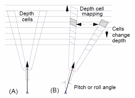
RDI ADCP data collected in Earth co-ordinates normally has had a depth cell mapping algorithm applied to align the depth cells to correct for tilt, while the other modes have not had it applied. Depth cell mapping is applied in post-processing in winADCP. Nortek's Storm / Surge post-processing software also applies bin-mapping when doing co-ordinate system rotations/transforms. (The term 'bin-mapping' is used by Nortek, RDI uses 'depth cell mapping'. We use 'bin-mapping' as it's the most common term in the literature.) Conversely, Nortek ADCP data collected in ENU co-ordinates has not had bin mapping applied. To apply bin-mapping, ENU data is converted back to Beam data, bin-mapping is applied and then converted back to ENU, doing any rotations as needed. The approach originated as described by Pulkkinen (1992). The Pulkkinen / RDI bin-mapping method is based on matching up the nearest vertical bin in each beam for each of the original range steps, then the radial velocities from those bins are used in the rotation to true Earth velocities. For compatibility with original VENUS ADCP data products, an alternative method is offered as a option as well, as described by Ott (2002). In that paper, the Ott method is shown to be an improvement over the discrete nearest vertical bin matching method. The Ott method uses a linear interpolation between the nearest vertical bins for each beam for each of the original range steps. The Ott method also interpolates over a small number of missing bins, otherwise missing data nullifies a greater extent of the data than it does in the nearest vertical bin method. The inner and outer most bins can end up with NaN values when there are less than 4 bins at the same vertical level, see the above graphic. This affects the nearest vertical bin method more so than the Ott method, and more bins are affected with increasing tilts.
Users are offered the option of 'None', 'Nearest vertical bin', or 'Linear interpolation (Ott method)'. When the data is in Earth co-ordinates, bin-mapping cannot be applied/modified. For RDI Earth data, the nearest vertical bin method has normally been applied, while Nortek Earth data does not have bin-mapping applied. In both cases, the users' preference may be overridden. The RDI manual indicates that pitch or roll values greater than 20 degrees are not possible and nominal processing has, in the past, applied NaN values when the pitch or roll exceeds that limit. However, we have found that RDI ADCPs can accurately report higher tilts. The limit is now set to 60 degrees for pitch/roll and at or above 90 degrees of average tilt, bin-mapping is overridden to the 'None' option.
Bin-mapping is not applied to the backscatter and intensity data. Instead, we offer a vertically corrected range in the mat file products and use this range for the plots when plotting against depth. For example, if the bin spacing is 1 m, but the tilt is 10 degrees, the vertical spacing is 0.98 m.
For advanced, interested users, here is the core code that does bin-mapping:
Three-Beam Solutions (For RDI ADCPs Only, Instr/Beam step #5)
In systems with four beams, the transformation from radial velocites to Earth co-ordinates velocities has redundant information; only three beams are needed to resolve currents in the three orthogonal directions, while the 4th beam effectively provides error estimation. In the case where exactly one bin out of of the four at any level is flagged and NaN'ed, then currents can still be calculated from the remaining three radial velocities, using the three-beam transformation solution. The screening steps that can flag the data 'NaN' prior to transformation include fish detection and correlation threshold, as well as any bin-mapping (particularly the RDI nearest vertical bin which can set many bins to NaN). The three-beam solution works by assigning the error velocity to be zero and then solving the transformation for the missing bin (for more details see Three Beam Solutions in adcp coordinate transformation_Jan08.pdf). With the missing data filled in, the normal transform from Beam to Instrument co-ordinate data is applied.
In cases where the data quality team has determined that an entire beam is bad, they can supply a device attribute specifying the bad beam number. That beam is then excluded in the processing from beam or instr co-ords and the values are filled in with the three-beam solution. Only the U,V,W results are affected, the raw velocity data as recorded by the instrument is presented without the exclusion. This forces the 3 beam option to on, regardless of the user input. The excluded beam number is mentioned in a comment on both the currents plot and intensity plots and in the processing comments in the mat files. This is currently only available for RDI ADCPs with 4 beams.
Here is the code for three-beam solutions and transform from Beam to Instrument (XYZ) co-ordinate data:
Screening
Correlation screening is the most widely applied and effective screening step, noted as step #3 in the Instr/Beam overall processing flow. It is also applied onboard RDI ADCPs when in Earth co-ordinate configuration, the value applied is available in the config structure.
Nortek ADCPs are generally three beam (so the three-beam solution option is not offered) and screening is not applied in the data products, except for a fixed 50% correlation screen on Nortek Signature55 data only, applied to match Nortek's Signature Viewer software.
RDI ADCPs screening steps also include a fish detection algorithm and screening, Instr/Beam step #4 in the overall process flow.
Once in Earth co-ordinates, the data can also be screened by the error velocity. Error velocity screening only applies to data with four valid beams (and non-zero error velocities). For further information on the screening steps, including algorithms, see adcp coordinate transformation_Jan08.pdf (RDI ADCPs only). This is step #9 in Instr/Beam and #2 in Earth data process flows.
Data Verification
As noted earlier, the ultimate requirement for the ADCP data products is that they replicate the results of the manufacturer's software. We test against the manufacturer's software to verify the data at every software release (regression testing). There are cases where this adherence is intentionally not true: if users choose any non-default option (or that says it's not the RDI default), the results will not match the default processing in the manufacturer's software, in particular, the Ott bin-mapping option is not available on winADCP at all. The testing suite includes manual and automated testing where the output of the manufacturer's software is compared to the data products and where data products are compared to the captured files from the previous release. The test suite is regularly updated for any new scenarios. Improvements in the test procedure are also made as needed. In addition to testing the software, there has been a significant effort to ensure that the metadata, in particular the heading metadata, is correct. These steps include careful measurement and documentation at deployment time, verifying and vetting ROV heading sensors, comparing data to nearby ADCPs, comparing results between various processing methods, and perhaps the best check is to compare the currents with the known/modelled tides. Contact us for information on the testing procedures and metadata verification.
A recent simplification in testing came about because of an improvement in the generation of RDI file data products, which we archive to speed up generation of subsequent products, MAT/NC files and plots. As of November 2015, RDI files with Beam or Instr co-ordinate data will incorporate the same heading/pitch/roll values as used for rotation and bin-mapping, that way, users and testers may load and process these files with RDI software, matching the values they can obtain from MAT and NC file products. For Earth co-ordinate data in RDI files, if we update the heading, we also need to rotate the East (u) and North (v) velocities as the new heading will be different from the internal compass heading (either fixed value, mobile position sensor or a magnetic declination is applied) on which the onboard Earth co-ordinate rotation was done. In this case, we don't update the pitch/roll as we cannot update the bin-mapping done for Earth data. Fortunately, the pitch/roll data is generally good and we do not yet have any examples where we do not use the internal pitch/roll data. Once the RDI files produced prior to November 2015 are re-generated, all RDI files will be made available in Data Search.
In all, the results from RDI winADCP, and Nortek software will match the processed data products. In addition, the original data, particularly the Beam co-ordinate data is always available in the RDI and Nortek raw binary files and as data.velocity (Nortek) and adcp.velocity (RDI) in the MAT files. The processingComments will completely describe the steps applied to produce the u,v,w processed velocities. In addition to the code snippets above, we are happy to supply more code, collaborate on that code, etc. We are interested in collaborating on QAQC processes, data verification, processing, analysis and research. Contact us if you have any questions.
Formats
Plots are available in PNG and PDF formats.
Oceans 3.0 API filter: extension={png,pdf}
Example:


Data Product Options For ADCPs (Ensemble averaging, bin-mapping, plan and plot limits)
![]()
Ensemble Period:
Data not altered (none)
Oceans 3.0 API filter: dpo_ensemblePeriod=0
1 Minute
Oceans 3.0 API filter: dpo_ensemblePeriod=60
10 Minute
Oceans 3.0 API filter: dpo_ensemblePeriod=600
15 Minute
Oceans 3.0 API filter: dpo_ensemblePeriod=900
1 Hour
Oceans 3.0 API filter: dpo_ensemblePeriod=3600
When selecting any of the ensemble periods, this option will cause the search to perform the standard box-car average resampling on the data. 'Boxes' of time are defined based on the ensemble period, e.g. starting every 15 minutes on the 15s, with the time stamp given as the center of the 'box'. Acoustic pings that occur within that box are averaged and the summary statistics are updated. This process is often called 'ping averaging'. The process uses log scale averaging on the intensity data, which involves backing out the logarithmic scale, compute the weighted average, and then compute the logarithmic scale again. Weighted averages are used when raw files bridge an ensemble period and when the data is already an ensemble or ping average.
New files are started when the maximum records per file is exceeded (usually set to make files that will use less than 1 GB of memory when loaded), or when there is a configuration, device or site changes. In the case where there is data from either side of a configuration change within the one ensemble period, two files will be produced with the same ensemble period, with the same time stamps, but different data. Users may use the ensemble statistics on the number of pings or samples per ensemble to filter out ensembles that do not have enough data. (As an aside, we do this by default with clean averaged scalar data - each ensemble period needs to have at least 70% of it's expected data to be reported as good.)
The default value is no averaging, meaning the data is not altered. This option is only available for MAT and NETCDF files.
File-name mode field
Selecting an ensemble period will add 'Ensemble' followed by the ensemble period. For example '-Ensemble600s'.
Velocity Bin-mapping (tilt compensation EX)
For all Nortek ADCP data products (PNG/PNG and MAT and netCDF formats)
![]()
This option specifies the bin-mapping processing method to be applied. Bin-mapping is also known as 'depth cell mapping' or 'tilt compensation' or even 'map to vertical'. There are two methods, both correct for tilt effects on ADCP velocity data, while the none option leaves the velocity data as is. For details on the two methods, see the section on correction and rotation of velocities (included below). The 'None' option is the default for Nortek ADCPs since the free version of the manufacturer's software does not apply bin-mapping (a core goal of our data products is to replicate the functionality offered by the manufacturer's software). The 'Nearest vertical bin' is the default for RDI ADCPs as winADCP applies this method for Instrument or Beam co-ordinate data. The 'As configured on the device' option uses the configuration onboard to determine whether to apply bin-mapping, this matches processing on-board the device (for Earth-co-ordinate data, while for Instrument or Beam co-ordinate data winADCP ignores the device configuration and always uses 'Nearest vertical bin'). The best method has been shown to be the linear interpolation method (Ott, 1992).
Nearest vertical bin
Oceans 3.0 API filter:
dpo_velocityBinmapping=1- As configured on the device (matches processing on device)
Oceans 3.0 API filter:dpo_velocityBinmapping=-1 None
Oceans 3.0 API filter: dpo_velocityBinmapping=0
Linear interpolation (Ott method)
Oceans 3.0 API filter: dpo_velocityBinmapping=2
File-name mode field
The velocity bin-mapping option will be appended to the filename. For example: '-binMapNone', 'binMapLinearInterp', 'binMapNearest'.
Nortek Signature Series Plan
For Nortek Signature Series ADCPs only, an additional option is appended to the above:
![]()
This option allows the user to select the specific data acquisition plan; there are two: PLAN and PLAN1. PLAN, also denoted as "PLAN0", is generally used for the base frequency (55 kHz), PLAN1 is the alternate (75 kHz). PLAN0 is always available, which is why it is the default option. If the device attribute AlternatePlanEnabled is true, and the DataFormat is DF3 (see the Nortek integrator's guide, DF3 is an internal setting), then PLAN1 data is available and may be accessed by the PLAN1 option. Otherwise requesting PLAN1 may result in no data found. Only appears to Nortek Signature Series ADCPs. When the alternate plan is active, the device will normally operate by alternating between the two frequencies, and the data products will respond by only including the data from the requested plan.
Normal PLAN (55 kHz)
Oceans 3.0 API filter: dpo_nortekSignatureSeriesPlan=0
Alternate PLAN1 (75 kHz if available)
Oceans 3.0 API filter: dpo_nortekSignatureSeriesPlan=1
All (55 kHz and 75 kHz if available)
Oceans 3.0 API filter:
dpo_nortekSignatureSeriesPlan='both'
File-name mode field
If the option is applied, a '-PLAN0' or a '-PLAN1' will be appended to the file-name.
Nortek Correlation Screen Threshold
For Nortek Signature Series ADCPs only, an additional option is appended to the above:
![]()
This option allows the user to control the correlation screening step. The default value retains the previous behaviour of ONC data products: a threshold of 50%. Beam-velocities that have associated correlation values lower than this threshold are are masked / screened to NaN values. Only available on Instrument or Beam co-ordinate data and Signature series ADCPs.
50% (Nortek default)
Oceans 3.0 API filter:corScreen=50Any percentage (integer between 1 and 100):
Oceans 3.0 API filter:corScreen=<1:100>Off (0%)
Oceans 3.0 API filter:corScreen=0
File-name mode field
If a value other than the default is used, a '-corr'<value> will be appended to the file-name, where <value> is the value of the option matching the API filter.
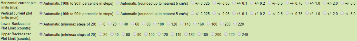
Horizontal / Vertical Current Plot Limits
This option allows the user to select automatic or fixed limits for ADCP daily current plots. The limits are on the colour axis of the daily current plots for either horizontal currents (East u, North v) or vertical currents (Up w) and are symmetric about zero (to support the diverging colour map, maintaining zero as white). The fixed limits have the benefit of being consistent from plot to plot, while the automatic limits can vary. The automatic (10th to 90th percentile) limit does attempt to maintain stable, suitable limits; the limit is selected from the same set of fixed limits that is available to the user by finding the limit that is greater than or equal to the 90th percentile of one-side horizontal or vertical current data. For both automatic limits, the data above the sea surface is excluded as it is often of extreme value.
Automatic (10th to 90th percentile in steps)
Oceans 3.0 API filter:dpo_horizontalcurrentplotlimits=0Automatic (rounded up to nearest 5 cm/s)
Oceans 3.0 API filter:dpo_horizontalcurrentplotlimits=-1+/- 0.025
Oceans 3.0 API filter:dpo_horizontalcurrentplotlimits=0.025+/- 0.05
Oceans 3.0 API filter:dpo_horizontalcurrentplotlimits=0.05+/- 0.1
Oceans 3.0 API filter:dpo_horizontalcurrentplotlimits=0.1+/- 0.2
Oceans 3.0 API filter:dpo_horizontalcurrentplotlimits=0.2+/- 0.5
Oceans 3.0 API filter:dpo_horizontalcurrentplotlimits=0.5+/- 0.75
Oceans 3.0 API filter:dpo_horizontalcurrentplotlimits=0.75+/- 1.0
Oceans 3.0 API filter:dpo_horizontalcurrentplotlimits=1.0+/- 2.0
Oceans 3.0 API filter:dpo_horizontalcurrentplotlimits=2.0+/- 5.0
Oceans 3.0 API filter:dpo_horizontalcurrentplotlimits=5.0
For the vertical current plot limits, substitute dpo_horizontalcurrentplotlimits with dpo_verticalcurrentplotlimits.
File-name mode field
Selecting a limit option other than 'Automatic (10th to 90th percentile)' or 'Automatic (no clipping, rounded up to nearest 5 cm/s)' will append to the file-name a '-Limit', following by the two limits selected, without the decimal point or trailing zeros. If one of the limits is Automatic (10th to 90th percentile in steps), 'Auto' will appear. If one of the limits is Automatic (rounded up to nearest 5 cm/s), AutoNoSat will appear. Examples: '-Limit0105', '-Limit021', '-Limit05Auto', '-LimitAuto5', '-LimitAutoNoSat5'.
Lower/Upper Backscatter Plot Limit
These options allow the user to select automatic or fixed limits for the colour scale of backscatter on the ADCP daily current plots. These options only affect the backscatter intensity plot (lowest panel). The lower and upper limits can be set independently. The fixed limits have the benefit of being consistent from plot to plot, while the automatic limits can vary. The automatic algorithm uses a 10/90 percent cumulative sum and quantizes to steps of 20 dB, making it much more stable than a simple min/max limit.
Automatic (min/max, steps of 20)
Oceans 3.0 API filter:backscatterLowerPlotLimits=-1 / backscatterUpperPlotLimits=-10
Oceans 3.0 API filter:backscatterLowerPlotLimits=020
Oceans 3.0 API filter:backscatterLowerPlotLimits=20 / backscatterUpperPlotLimits=20... (options in steps of 20 dB)200
Oceans 3.0 API filter:backscatterLowerPlotLimits=200 / backscatterUpperPlotLimits=200220
Oceans 3.0 API filter:backscatterUpperPlotLimits=220
Backscatter Colour Map
For Nortek and RDI ADCP daily current plot products (PNG and PDF formats) and echosounder backscatter plots (ASL, BioSonics)
This option allows the user to select the colourmap used for the backscatter plot. An example of each colourmap available is displayed below, along with the Oceans 3.0 API filter for that specific colourmap.
Default (ONC/VENUS rainbow/jet colours)
Oceans 3.0 API filter:
dpo_backScatterColourmap=0
Modified Default (perceptually smooth rainbow/jet colours from m_map toolbox)
Oceans 3.0 API filter:
dpo_backScatterColourmap=1
Sourced from: Pawlowicz, R., 2019. "M_Map: A mapping package for MATLAB", version 1.4k, [Computer software], available online at www.eoas.ubc.ca/~rich/map.html.
Sequential Blue to Purple (perceptually balanced - from colorbrewer.org)
Oceans 3.0 API filter:
dpo_backScatterColourmap=2
Sourced from: Charles (2020). cbrewer : colorbrewer schemes for Matlab (https://www.mathworks.com/matlabcentral/fileexchange/34087-cbrewer-colorbrewer-schemes-for-matlab), MATLAB Central File Exchange. Retrieved January 7, 2020.
Sequential Red to Yellow (perceptually balanced - from colorbrewer.org)
Oceans 3.0 API filter: dpo_backScatterColourmap=3

Sourced from: Charles (2020). cbrewer : colorbrewer schemes for Matlab (https://www.mathworks.com/matlabcentral/fileexchange/34087-cbrewer-colorbrewer-schemes-for-matlab), MATLAB Central File Exchange. Retrieved January 7, 2020.
Sequential Blue to Yellow (perceptually balanced - MATLAB Parula)
Oceans 3.0 API filter:
dpo_backScatterColourmap=4
Diverging Spectral (perceptually balanced - from colorbrewer.org)
Oceans 3.0 API filter:
dpo_backScatterColourmap=5
Sourced from: Charles (2020). cbrewer : colorbrewer schemes for Matlab (https://www.mathworks.com/matlabcentral/fileexchange/34087-cbrewer-colorbrewer-schemes-for-matlab), MATLAB Central File Exchange. Retrieved January 7, 2020.
Discussion
To comment on this product, click Add Comment below.